https://doi.org/10.5194/gi-6-439-2017
© Author(s) 2017. This work is distributed under the Creative Commons Attribution 3.0 License.
Fog-based automatic true north detection for absolute magnetic
declination measurement
Alexandre Gonsette, Jean Rasson, Stephan Bracke, Antoine Poncelet, Olivier Hendrickx, and François Humbled Dourbes magnetic observatory, Royal Meteorological Institute of Belgium, Dourbes, 5670, Belgium
Correspondence to:Alexandre Gonsette ([email protected]) Received: 3 March 2017 – Discussion started: 24 April 2017
Revised: 29 August 2017 – Accepted: 10 September 2017 – Published: 26 October 2017
Abstract.Absolute magnetic measurements are of great im-portance in magnetic observatories. They allow not only in-strument calibration but also data quality checking. They re-quire the vertical and the geographic or true north as refer-ence directions, usually determined by means of a level and by pointing an azimuth mark, respectively. We present here a novel system able to measure the direction of the magnetic field and of the vertical and true north. A design of a north seeker is proposed taking into account sensor bias as well as misalignment errors. Different methods are derived from this model and measurement results are presented. A measure-ment test at high latitude is also shown.
1 Introduction
Measuring the magnetic declination is realized by determin-ing, in a horizontal plane, both magnetic field and geographic or true north direction (in the rest of this paper, the term true north will be employed). Then the angle between them is computed. In magnetic observatory as well as in the field, this value is measured by an observer during the so-called “absolute” measurement step (Rasson, 2005). This procedure consists of two main steps in manipulating a DI-flux instru-ment. First, the instrument is oriented relative to the mag-netic field in order to establish its direction in space. Practi-cally, the magnetic field sensor mounted on the telescope is placed in the horizontal plane. The sensor output is then the projection of the field horizontal component along the sensor sensitive axis or, in other words, the scalar product of both. The most sensitive direction is therefore perpendicular to the magnetic field. Then, the true north is determined by pointing at a target whose azimuth is already known. Finally the
ob-server extracts the magnetic declination from both readings. The target azimuth can be established by different methods: by a gyrotheodolite, by pointing at a celestial body such as the Sun in combination with a clock or by using a GNSS system (Newitt et al., 1996). In any case, this target azimuth value is measured prior to the declination measurement and is assumed constant until it is checked again.
2 Background
A fiber-optic gyroscope (FOG) is an absolute rotation sensor and may be able to detect the Earth’s rotation. Its principle is based on the Sagnac effect (Arditty and Lefèvre, 1981). Briefly, let us imagine two balls rolling at the same speed but in opposite directions at the circumference of a disc. If the disc is static, an external observer would see both balls crossing each other after half a turn and again at the start point. If the disc is put into rotation, the balls will not reach the start point relative to an inertial frame at the same time. The delay is therefore proportional to the disc rotation speed. FOG-based sensors use a similar principle: two light beams traveling at the same speed along an optical fiber are in-jected from each end. The phase shift between the two optical waves gives the sensor rotation speed.
2.1 Static method
North seeker methods are usually sorted in two categories: static (Liu et al., 2014) and dynamic (Xu and Guo, 2010). In both cases, the sensitive axis of the FOG is directed horizon-tally and the projection of the Earth’s rotation vector on it is given by
ω (φ) =ecos(θ )cos(φ)+b, (1) whereωis the angular speed recorded by FOG,φis the angle between true north and the direction pointed by the FOG’s sensitive axis, θ is the latitude, e is the Earth’s rotation speed∼15.041◦h−1, andbis the FOG bias.
In the static method, two opposite directions are pointed in order to compensate for the bias. Due to the cos(φ)term, the most sensitive directions lie along the east–west axis. The true north is then found by adding or removing 90◦ from the result. Additional pointing close to the east–west may be required so that the FOG sensor scale factor can be cal-ibrated. For automatization purpose, it is possible to point at still more directions in order to remove the east–west uncer-tainty.
ω1(φ)=ecos(θ )cos(φ)+b,
ω2(φ+π )=ecos(θ )cos(φ+π )+b, φ=acos
ω
1−ω2 2ecos(θ )
+wn, (2)
wherewnis an instrumental white noise. The previous equa-tion suggests to increase the sampling time in order to re-duce the white noise. However, the bias is subject to drift due to environmental changes like temperature. The prob-lem is therefore to find the optimum sampling time that min-imize both white noise and drift contribution to uncertainty. The Allan variance is a useful tool for this. Since the FOG remains stationary during each acquisition step its output is supposed to remain constant. The minimum in the curve of the Allan variance gives the optimum acquisition time as well as the uncertainty level of measurement.
2.2 Dynamic and combined method
In the dynamic method, the FOG’s sensitive axis is also kept horizontal but continuously turns around a vertical axis. The phase shift of the FOG output gives the true north direction (±90◦) with respect to the arbitrary zero of the angle reading in the instrument frame. This method is not affected by the sensor bias so that at first glance it could be preferred to the static one. Unfortunately the sensitivity of FOG sensors is too low to allow this dynamic method to be used for azimuth determination in the particular case of magnetic declination measurement.
It is also possible to combine both methods by perform-ing static measurements at regularly spaced angular positions (Abbas, 2013). In this hybrid case, the sampling time can be optimum. The output is therefore a discrete sinus curve whose amplitude is given byecos(θ ). The phase shift gives the true north direction (±90◦).
3 New approach
The above true north methods do not consider a possible FOG misalignment. However, it is evident that a horizon-tal misalignment has a direct impact on the measurement. Again, since the sensor is supposed to measure the horizontal component of the Earth’s rotation vector (see Eq. 1), a verti-cal misalignment also leads to an error due to the orthogonal projection of vertical component of the Earth’s rotation vec-tor onto the plane of measurement of the FOG sensor. Many FOG-based north seekers only have the possibility to rotate around the vertical axis so that they do not have the opportu-nity to take misalignment into account. When looking to the accuracy of magnetic declination required by international standards like those established by Intermagnet (Intermag-net, 2012), it appears evident that such error must be com-pensated. Indeed, the 5 nT maximum allowed error on theY component leads to a maximum misalignment error (case in Dourbes withHm=20 µT):
Misalignment error=180
π atan
5
20 000
=0.014◦. (3) Reciprocally, a small 0.05◦misalignment error would corre-spond to 17.5 nT.
3.1 GyroDIF
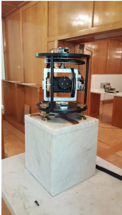
Figure 1.GyroDIF instrument.
The GyroDIF instrument is a non-magnetic robotized plat-form able to orient sensors in any direction. It is based on the AutoDIF system. A fluxgate sensor and a FOG are mounted on the horizontal axis. Neglecting misalignment errors, both have their sensitive direction parallel. Piezoelectric motors can rotate the horizontal and vertical axes with a resolu-tion up to 0.001◦. An electrolytic level continuously records tilt errors with 0.1 arcsec resolution and 1 arcsec linearity. Non-magnetic angular encoders allow angles measurement with accuracy better than 6 arcsec according to ISO 17-123 (Gonsette et al., 2014). The angle readings respect the DI-flux conventions with a horizontal circle increasing clock-wise and a vertical circle such that zero is read when fluxgate is roughly vertical and+90◦when fluxgate is horizontal on top of the axis (commonly sensor up). Figure 1 presents the GyroDIF implementation.
3.2 An extended model
In the middle of the 1980s, Kring Lauridsen (Lauridsen, 1985) and David Kerridge (Kerridge, 1988) established a model mathematically describing the magnetic field vec-tor in the DI-flux sensor reference frame. The theodolite was supposed to have 2 degrees of freedom, perfectly leveled and free of mechanical errors such as orthogonality errors or play in axes. They included a sensor offset and two angles describ-ing the misalignment of the fluxgate sensitive axis relative to the telescope optical axis. Kerridge model leads to the fol-lowing equation:
T =Hcos(φ−D)(cos(β)−sin(β))−γ Hsin(φ−D)
+Z(sin(β)+cos(β))+T0, (4) where H, Z and D are the geomagnetic horizontal, verti-cal and declination components, respectively;andgamma are the vertical and horizontal sensor misalignments, respec-tively;T andT0 are the sensor output and offset, respec-tively;φ and β are the rotation angles around the vertical and horizontal axes relative to true north and horizontal, respectively. From the previous equation, Kerridge derived a method based on four measurements that led to a final dec-lination measurement result free of those three errors (at first order). Similar development has been performed for mag-netic inclination.
However, considering a platform like the GyroDIF with two orthogonal rotation axes, a similar model can be imple-mented. Furthermore, this system also records its tilt angle, which could be modeled by 2 angular degrees of freedom. The Earth’s rotation vector can be expressed in the FOG sen-sor reference frame withzaxis in the sensor axis direction and considering small tilt and misalignment angles:
ω=
1 0 −g
0 1 γg
g −γg 1
Ry(β) Rx(φ)
×
1 B −A
−B 1 0 A 0 1
cos(θ ) 0 −sin(θ )
0 1 0
sin(θ ) 0 cos(θ )
×
0 0 e
+
Tx Ty Tz
, (5)
whereTxyzis the sensor offset in theX, Y andZdirection,A andBare the northward and eastward tilt angles,Rx,y(X)is the elementary rotation matrix around localxandyaxes,φis the angle between true north and the sensor axis (neglecting misalignment angles),β is the angle between the horizon-tal plan and sensor axis (neglecting misalignment angles),g is the FOG misalignment in the vertical plane andγgis the FOG misalignment in the horizontal plane.
the Kerridge model is evident. Only the leveling terms are added.
ω3≈Hecos(φ) cos(β)−gsin(β)−γgHesin(φ)
−Ze sin(β)+gcos(β)
−Zecos(β) (Acos(φ)+Bsin(φ))+Tz, (6) whereHe=ecos(θ )andZe=esin(θ ).
3.3 Four-position method
The static method can be adapted in order to compensate for the FOG misalignment. For an arbitrary direction φ, Eq. (6) leads to four equations. Small angle approximations are made forβ≈0 andβ≈π:
ω3a(φ, β=0)≈Hecos(φ)−γgHesin(φ)
−Ze βa+g−Ze(Acos(φ)+Bsin(φ))+Tz, (7) ω3b(φ, β=π )≈ −Hecos(φ)−γgHesin(φ)
+Ze βb+g
+Ze(Acos(φ)+Bsin(φ))+Tz, (8) ω3c(φ+π, β=π ) ≈Hecos(φ)+γgHesin(φ)
+Ze βc+g−Ze(Acos(φ)+Bsin(φ))+Tz, (9) ω3d(φ+π, β=0)≈ −Hecos(φ)+γgHesin(φ)
−Ze βd+g+Ze(Acos(φ)+Bsin(φ))+Tz. (10) Combining Eqs. (7) to (10), almost all errors vanish at first order. It is reasonable to consider the horizontality errorsZeβ as random errors that also vanish while the number of mea-surements increases. The resulting angular speed is
ωr =ωa−ωb+ωc−ωd
4
≈Hecos(φ)−Ze(Acos(φ)+Bsin(φ)) . (11) The last term corresponds to the leveling error monitored by the electronic level. The angle relative to true north is then given by
φ=acos
ωr He
+tan(θ ) (Acos(φ)+Bsin(φ))
. (12) From Eq. (12), the optimum measurement direction is the east–west axis (φ≈90◦). In this case, the resulting angu-lar speed is close to zero in the quasi-linear part of the co-sine function. However, Eq. (12) does not take into account a possible scale factor uncertainty. The sensor output is usu-ally a voltage or a digital value that need to be converted in corresponding angular speed. An error in ωr introduces an error in the true north determination. To reduce this effect a solution consists of performing two sets of four measure-ments at two close but different directions and then finding the corresponding zero position by interpolation.
3.4 Hybrid method
The four- (or eight-) position method requires to roughly know a priori the true north direction. Moreover, instrument uncertainties (angular sensors and FOG) will cause an error even with an interpolation procedure. Comparatively a hy-brid method combining static and dynamic methods ranges the whole circle and performs a measurement at regular inter-vals (e.g., each 10◦). At each angular position a four-position set of measurement is executed, leading to a resulting angular speed given by Eq. (11). A sinus linear least-squares fitting is then applied on the discrete sinus data according to Ras-son (2009).
There are different ways to implement the hybrid method in the case of GyroDIF. For instance, we can choose to per-form all measurements withhaxis at 90◦and then the mea-surements withhaxis at 270◦. This would lead to two sine curves. The first one corresponds to sensor up while the sec-ond one is recorded after rotating theh axis by 180◦. The resulting phase shift is finally the mean phase of both sinus fitted curves. Another possibility is to take advantage of the static method by performing four measurements at each step. Thus only one resulting discrete sinus curve is recorded.
4 Results
4.1 Interpolated four-position method
The interpolated four-position method has been tested first. A cost-effective FOG has been used for validating the theory. The optimum acquisition time and bias stability have been defined from Allan variance (Fig. 2). They are, respectively, 500 s and 0.05◦h−1. Two positions around the eastern direc-tion have been arbitrarily defined. The instrument has been installed in the absolute house of Dourbes magnetic obser-vatory. Like conventional DI-flux, GyroDIF has been placed on a geodetic pillar. A “low level” of thermal stability has been established. Room temperature is controlled by means of a standard thermal regulator so that temperature changes are not worse than 2 or 3◦peak to peak and an insulated en-closure (10 cm thick extruded polystyrene) has been placed around the device. A series of more than 1800 measurements is presented in Fig. 3.
Standard deviation (SD) is about 1σ≈0.1◦, which is clearly too much compared to the international standard. Nevertheless, this dispersion appears to be a white noise and thus, when the number of samples is sufficient (here N=1800), the final uncertainty can be reduced to
σN= σ
√
N
≈0.0024◦. (13)
Figure 2.Allan variance plot giving the FOG output SD according to the acquisition time. The minimum value gives the bias stability and the acquisition optimum time.
Figure 3.Long-term series of interpolated four-position gyro-north-seeker measurement (trace on horizontal circle).
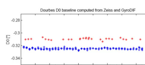
thanks to the measurement protocol. This is the case if and only if we do not take into account the instrument uncertain-ties and a possible FOG nonlinearity, e.g., injection locking or pulling effects (Razavi, 2004). For this last, Eq. (12) sug-gests that 100 ppm would lead to 20 arcsec error. Figure 4 presents Dourbes LAMA variometer D0 baseline (Rasson, 2005) computed from GyroDIF and conventional DI-flux ab-solute measurements. Both measurements are separated by a small 0.01◦offset that would correspond to 3.5 nT on theY component.
The presence ofθin Eqs. (6) and (11) shows that the north-seeking sensitivity decreases as the latitude increases. Actu-ally, the problem is similar to measuring magnetic declina-tion at high magnetic latitude where the horizontal compo-nent is weak. If we consider that automatic observatories are desirable in the polar regions, testing the sensitivity at high latitude becomes crucial. This is why a series of measure-ments has been made in Sodankylä magnetic observatory, latitude 67◦220N. The observed SD in the north-seeking pro-cedure is 1σ ≈0.16◦, which is more than in Dourbes but still manageable. Figure 5 presents the result of interpolated four-position measurements in Sodankylä.
Figure 4.Baseline D0 comparison. Blue dots are computed from GyroDIF measurements. Red dots are computed from conventional DI-flux instrument (Zeiss 010-B).
4.2 Remarks on absolute magnetic declination measurement accuracy
sta-Figure 5.Series of true north measurements (trace on horizontal circle) at Sodankylä magnetic observatory. The angle readings cor-respond to horizontal circle value when instrument is pointing true north.
Figure 6.Result of the intercomparison session organized during the XVIIth IAGA Workshop on Geomagnetic Observatory instru-ments, data Acquisition and Processing. Each value corresponds to the mean result of an observer/instrument series performed on pillar D05. Eastern componentY0 is shown.
tistical value computed over a whole turn while the four-position method always uses the same four-positions, leading to a systematic error that could be slightly different from the statistical one. In the case of conventional measurements, the observer’s eyesight and ability to point the target in the same way as a colleague is seldom better than 5 arcsec and also depends on the telescope optics. Other sources of uncer-tainty are the pillar difference; time synchronization between variometer and absolute instrument, including scalar instru-ment; and magnetic cleanliness of the absolute room or the observer. It should be noted that intercomparing absolute in-struments by performing parallel measurements using a var-iometer baseline as a yardstick rarely secures accuracies bet-ter than±10 arcsec for magnetic declination. The intercom-parison session organized during XVIIth IAGA Workshop on Geomagnetic Observatory Instruments, Data Acquisition and Processing gives an idea of the usual baseline difference ob-tained from different couples of instruments and observers. For instance, 25 participants performed a series of absolute measurement on pillar D05 (other participants measured on other pillars). The mean value of each participant series is shown on Fig. 6. Most of the results are within±2 nT. 4.3 Hybrid method
The hybrid method has also been implemented. A four-position protocol is executed every 10◦, starting from 5 to
Figure 7.Fiber-optic gyro output signal due to Earth’s rotation when its sensitive axis scans the horizontal plane in Dourbes. The maximum of the sine function corresponds to true north. Blue: hy-brid methodωr according to Eq. (11). Red: sinus fitting.
Figure 8.Series of true north measurements (trace on horizontal circle) obtained by means of hybrid method (Dots). The solid line corresponds to the true north determination after passing through a Kalman filter.
355◦on the horizontal circle (i.e., around the vertical axis). The whole procedure therefore requires 144 measurements. Figure 7 shows the 36 resulting measurements according to Eq. (11) and the corresponding sinus fitting. In order to keep reasonable measurement duration, FOG signal acquisition time has been reduced to 45 s per position. Adding the mo-tion time and stabilizamo-tion time for the bubble level, the entire protocol takes about 2 h.
The series of measurements presented in Fig. 8 has an SD 1σ≈0.06◦. Because we cannot exclude the possibility that the pillar and the instrument resting on it may change its ori-entation over the time, we must be able to track this long-term angular variation. Therefore a low-pass filter must be implemented. It could be a sliding mean but it is common to use a Kalman filter when working with FOG. In this case, the filtered values have a SD 1σ ≈0.004◦.
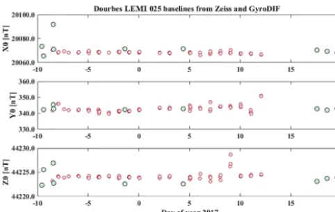
Figure 9.Blue: Dourbes LEMI 025 baselines computed from Gy-roDIF measurements (red). The true north direction used in theY0 baseline is determined by means of hybrid method. The green dots are computed from conventional DI-flux measurements.
Sect. 4.1 since the difference inY0 is within 1 nT. However, we should note that the number of measurement is limited to 3 weeks. Also only a few comparative conventional mea-surements have been performed. Nevertheless, as explained in Sect. 4.2, the systematic errors due to angle reading are clearly reduced due to the higher amount of steps.
5 Conclusion
In this paper, we presented a new improvement in automation of magnetic observatories. Different methods for automati-cally finding true north have been established and demon-strated. It appears that the hybrid method is more in accor-dance with the concept of an automatic setup. Moreover, a se-ries of instrument uncertainties are smoothed during the sinus fitting step. Results presented here have been obtained with a low-cost FOG sensor. A more sensitive device may lead to better and faster result. In particular, high-latitude observa-tories need accurate FOG asHethen becomes small. Never-theless, measurements made at Dourbes observatory already meet Intermagnet accuracy standards.
Data availability. Data are available upon request from the corre-sponding author at [email protected].
Competing interests. The authors declare that they have no conflict of interest.
Special issue statement. This article is part of the special issue “The Earth’s magnetic field: measurements, data, and applications from ground observations (ANGEO/GI inter-journal SI)”. It is a re-sult of the XVIIth IAGA Workshop on Geomagnetic Observatory
Instruments, Data Acquisition and Processing, Dourbes, Belgium, 4–10 September 2016.
Acknowledgements. We would like to acknowledge the Royal Meteorological Institute of Belgium, which allowed this research. We also acknowledge the editor and the reviewers who contributed to the improvement of this article.
Edited by: Kusumita Arora
Reviewed by: Heinz-Peter Brunke and Christopher Turbitt
References
Abbas, A.: Design and implementation of FOG based gyrocompass, Appl. Mech. Mater., 332, 124–129, 2013.
Arditty, H. J. and Lefèvre, H. C.: Sagnac effect in fiber gyroscopes, Opt. Lett., 6, 401–403, 1981.
Auster, H.-U., Mandea, M., Geese [Hemshorn], A., Korte, M., and Pulz, E.: Automation of absolute measurement of the geomagnetic field, Earth Planet. Space, 59, 1007–1014, https://doi.org/10.1186/BF03352041, 2007.
Eckstaller, A., Müller, C., Ceranna, L., and Hartmann, G.: The geophysics observatory at Neumayer stations (GvN and NM-II) Antarctica, Polarforschung, 76, 3–24, 2007.
Gilbert, D. and Rasson, J. L.: Effect on DIFlux measuring accuracy due to a magnet located on it, in: Proceeding of the VIIth IAGA workshop on geomagnetic observatory instrument, data acquisi-tion and processing, 8–15 September 1996, Niemegk, Germany, 1998.
Gonsette, A., Poncelet, A., Marin, J.-L., Bracke, S., and Ras-son, J. L.: Autodif validation procedure, in: Proceeding of the XVIth IAGA workshop on geomagnetic observatory instrument, data acquisition and processing, 7–16 October 2014, Hyderabad, India, 2014.
Kerridge, D. J.: Theory of the fluxgate-theodolite, Report WM/88/14, British Geological Survey, 1988.
Lauridsen, E. K.: Experience with the Declination-Inclination (DI) Fluxgate Magnetometer Including Theory of the Instrument and Comparison with other Methods, Geophysical Papers, R-71, Danish Meteorological Institute, Copenhagen, 1985.
Liu, Y., Liu, S., Wang, C., and Wang, L.: A new North-seeking method based on MEMS gyroscopes, Sensor & Transducers, 178, 14–19, 2014.
Marsal, S., Curto, J. J., Torta, J. M., Gonsette, A., Favà, V., Ras-son, J., Ibañez, M., and Cid, Ò.: An automatic DI-flux at the Livingston Island geomagnetic observatory, Antarctica: require-ments and lessons learned, Geosci. Instrum. Method. Data Syst., 6, 269–277, https://doi.org/10.5194/gi-6-269-2017, 2017. Newitt, L. R., Barton, C. E., and Bitterly, J.: Guide for Magnetic
Repeat Station Surveys, IAGA, Boulder, USA, 1996.
Poncelet, A., Gonsette, A., and Rasson, J.: Several years of ex-perience with automatic DI-flux systems: theory, validation and results, Geosci. Instrum. Method. Data Syst., 6, 353–360, https://doi.org/10.5194/gi-6-353-2017, 2017.
Tech-nique No 040, Institut Royal Meteorologique de Belgique, Brus-sels, 43 pp., 2005.
Rasson, J. L.: Testing the time-stamp accuracy of a digital variome-ter and its data logger, in: Proceedings of the XIIIth IAGA Work-shop on geomagnetic observatory instruments, data acquisition, and processing, US Geological Survey Open-File Report 2009– 1226, 225–231, 2009.
Rasson, J. L. and Gonsette, A.: The Mark II Auto-matic Diflux, Data Sci. J., 10, IAGA169–IAGA173, https://doi.org/10.2481/dsj.IAGA-24, 2011.
Razavi, B.: A study of injection locking and pulling in oscillators, IEEE J. Solid-St. Circ., 39, 1415–1424, https://doi.org/10.1109/JSSC.2004.831608, 2004.
St-Louis, B. J.: INTERMAGNET Technical Reference Manual, V4.6, INTERMAGNET, available at: http://www.intermagnet. org/publication-software/technicalsoft-eng.php (last access: 25 October 2017), 2012.