Molecular Dynamics and X-ray Powder Diffraction Simulations: Investigation of nano-polycrystalline microstructure at the atomic scale coupling local structure configurations and X-ray powder Diffraction techniques

Doctoral School in Materials Science and Engineering

M

M

o

o

l

l

e

e

c

c

u

u

l

l

a

a

r

r

D

D

y

y

n

n

a

a

m

m

i

i

c

c

s

s

a

a

n

n

d

d

X

X

-

-

r

r

a

a

y

y

P

P

o

o

w

w

d

d

e

e

r

r

D

D

i

i

f

f

f

f

r

r

a

a

c

c

t

t

i

i

o

o

n

n

S

S

i

i

m

m

u

u

l

l

a

a

t

t

i

i

o

o

n

n

s

s

I

In

nv

ve

es

st

ti

i

ga

g

at

ti

i

on

o

n

o

of

f

na

n

an

no

o-

-p

po

ol

ly

yc

cr

r

ys

y

s

ta

t

al

ll

l

in

i

ne

e

m

mi

ic

cr

ro

os

st

tr

ru

uc

ct

t

ur

u

r

e

e

a

at

t

t

t

he

h

e

a

at

to

om

mi

ic

c

s

sc

ca

al

l

e

e

c

co

ou

up

pl

l

in

i

ng

g

l

l

o

o

c

c

a

a

l

l

s

s

t

t

r

r

u

u

c

c

t

t

u

u

r

r

e

e

c

c

o

o

n

n

f

f

i

i

g

g

u

u

r

r

a

a

t

t

i

i

o

o

n

n

s

s

a

an

nd

d

X

X

-

-

r

r

a

a

y

y

P

P

o

o

w

w

d

d

e

e

r

r

D

D

i

i

f

f

f

f

r

r

a

a

c

c

t

t

i

i

o

o

n

n

t

te

ec

ch

hn

ni

iq

qu

ue

es

s

Alberto Leonardi

November 2012

X

X

IV

c

yc

M

OLECULAR

D

YNAMICS AND

X-

RAY

P

OWDER

D

IFFRACTION

S

IMULATIONS

I

-

AND

X-

D

Alberto Leonardi

E-mail: [email protected]

Approved by:

Department of Materials Engineering and Industrial Technologies University of Trento, Italy.

Prof. Matteo Leoni

Department of Materials Engineering and Industrial Technologies University of Trento, Italy.

Ph.D. Commission:

Department of Materials Engineering and Industrial Technologies University of Trento, Italy.

Prof. Rozalya Barabash

Materials Science & Technology Div. Oak Ridge National Laboratory, Tenneesee (US).

Prof. Marco Milanesio

Department of Science and advanced technologies

University of Piemonte Orientale, Italy.

University of Trento, faculty of engineering

Department of Materials Engineering and Industrial Technologies

University of Trento - Department of

Materials Engineering and Industrial Technologies

Doctoral Thesis

Alberto Leonardi - 2012

Published in Trento (Italy) – by University of Trento

"The essence of science lies not in discovering facts, but in

discovering new ways of thinking about them. “

Abstract

Atomistic simulations based on Molecular Dynamics (MD) were used to model the lattice distortions in metallic nano-polycrystalline microstructures, with the purpose of supporting the analysis of the X-ray powder diffraction patterns with a better, atomic level understanding of the studied system.

Complex microstructures were generated with a new modified Voronoi tessellation method which provides a direct relation between generation parameters and statistical properties of the resulting model. MD was used to equilibrate the system: the corresponding strain field was described both in the core and in surface regions of the different crystalline domains. New methods were developed to calculate the strain tensor at the atomic scale.

Line Profile Analysis (LPA) was employed to retrieve the microstructure information (size and strain effects) from the powder diffraction patterns: a general algorithm with an atomic level resolution was developed to consider the size effects of crystalline domains of any arbitrary shape. The study provided a new point of view on the role of the grain boundary regions in nano-polycrystalline aggregates, exploring the interference effects between different domains and between grain boundary and crystalline regions. Usual concepts of solid mechanics were brought in the atomistic models to describe the strain effects on the powder diffraction pattern. To this purpose the new concept of Directional - Pair Distribution Function (D-PDF) was developed. D-PDFs calculated from equilibrated atomistic simulations provide a representation of the strain field which is directly comparable with the results of traditional LPA (e.g. Williamson-Hall plot and Warren-Averbach method).

Table of contents

Chapter I

Introduction ... 13

Chapter II

Modelling of Material Microstructures ... 17

2.1.

Abstract ... 17

2.2.

Introduction ... 18

2.3.

Methods ... 20

2.3.1.

Traditional stochastic tessellation methods ... 20

2.3.2.

Modified Voronoi Tessellation (MVT) ... 22

2.3.2.1.

Relationships between traditional tessellations and the MVT

... 25

2.3.3.

Constrained Modified Voronoi Tessellation (CMVT) ... 27

2.4.

Results and discussion ... 28

2.4.1.

Atomic density and voids in MVT-derived microstructures .. 28

2.4.2.

Statistical properties of the MVT ... 32

2.4.3.

Relationship between input parameters and resulting

microstructure ... 36

2.4.4.

Reliability of MVT statistics by the evolutionary CMVT ... 39

2.4.5.

Multiple target properties optimization with CMVT ... 41

2.4.6.

MVT computing performance ... 44

2.5.

Conclusion ... 46

Chapter III

Analysis of Atomistic Simulation Data ... 47

3.1.

Abstract ... 47

3.2.

Introduction ... 48

3.3.

Methods ... 49

3.3.1.

Molecular Dynamics simulation ... 49

3.3.3.

Local coordination and surface shape ... 52

3.3.4.

Strain at the atomic level ... 54

3.3.4.1.

The Voronoi Cell Deformation method (VCD) ... 55

3.3.4.2.

The evolutional Voronoi Cell Deformation method (eVCD)

... 56

3.3.5.

Isotropic and Anisotropic strains ... 57

3.3.6.

Potential energy and Stress at the atomic level ... 59

3.4.

Results and discussion ... 60

3.4.1.

Strain at the atomic level in a nano-polycrystalline microstructure

from MD ... 60

3.4.2.

Stress – Strain relation in polycrystalline microstructure ... 68

3.4.3.

Preliminary X-ray Diffraction Line Profile analysis ... 70

3.5.

Conclusion ... 73

3.6.

Appendix III.A:

Deformation of convex polyhedron from volume properties

... 74

3.7.

Appendix III.B:

Deformation of convex polyhedron from mass properties

... 76

Chapter IV

Interference Effects in Nano-crystalline Systems ... 77

4.1.

Abstract ... 77

4.2.

Introduction ... 78

4.3.

Generation of the nano-polycrystalline model ... 78

4.4.

Results and Discussion ... 79

4.5.

Conclusions ... 86

Chapter V

Common Volume Function & Diffraction Line Profiles ... 87

5.1.

Abstract ... 87

5.2.

Introduction ... 88

5.3.1.

Convex polyhedra ... 90

5.3.2.

Non-convex polyhedra ... 93

5.4.

Examples of application ... 93

5.4.1.

Convex shapes ... 94

5.4.1.1.

Truncated and bitruncated cube ... 94

5.4.1.2.

Irregular domain shapes: 3D Voronoi cell ... 95

5.4.1.3.

Polycrystalline microstructure: 3D Poisson-Voronoi

microstructure ... 97

5.4.2.

Non-convex shapes ... 98

5.4.2.1.

Planar tripods and tetrapods ... 98

5.4.2.2.

Hollow cubes ... 100

5.4.3.

Non-polyhedral shapes ... 102

5.5.

Conclusions ... 104

5.6.

Appendix V.A:

Common Volume Function in the frame of set theory ... 105

Chapter VI

Directional - Pair Distribution Function ... 107

6.1.

Abstract ... 107

6.2.

Introduction ... 108

6.3.

Cupper nano-polycrystalline microstructure: generation and

strain distribution ... 109

6.3.1.

Directional - Pair Distribution Function (D-PDF)... 112

6.3.2.

Powder pattern from a nano-polycrystalline microstructure. 116

6.3.3.

D-PDF and r.m.s strain ... 120

6.4.

Conclusions ... 130

List of abbreviation and acronyms ... 133

References ... 137

Scientific Production ... 151

Participation to Congresses, Schools and Workshops ... 152

Implemented algorithms ... 153

Chapter I

Introduction

Computational Materials Science is one of the newest and most promising branches of science and engineering. Owing to their versatility, computational techniques can be employed both to assess consistency between experiments and theories, and to complement them. For example, predictions can be made by using different models or by implementing different hypothesis, so to find the best experimental conditions under which some known, or new and unexpected phenomena appear ( (Zheng, et al., 2010), (Bulatov, et al., 1998), (Greaves, et al., 2011), (Jang, et al., 2012), (Norris, et al., 2011)).

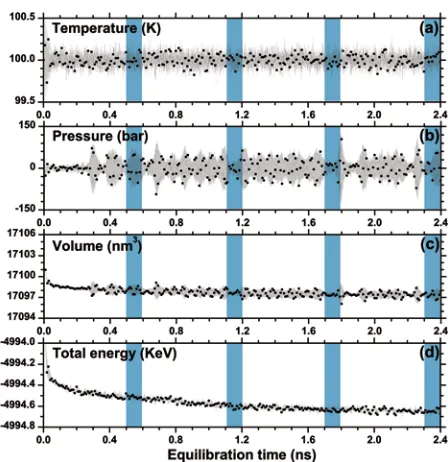
The increasing power of computers is constantly pushing up the capabilities and limits of MD: ever larger clusters of atoms (i.e. microstructures), can be nowadays equilibrated under a wide variety of imposed environmental conditions. One million atoms can easily be handled by a desktop PC, whereas computer clusters are usually employed for more demanding tasks (several hundred million atoms). Still, transient phenomena are frequently poorly traced (Van Swygenhoven, 2002) and thus the risk is high of a strong biasing of the result by a wrong choice of the starting microstructure. Hence, it is crucial that statistical and physical coherency is kept between simulated microstructure and (as available) experimental results ( (Gross, et al., 2002), (Xu, et al., 2009), (Xu, et al., 2010)).

A convenient way to link atomistic simulations and experiments is based on X-ray powder diffraction. In fact, a diffraction pattern contains complete information on a nano-crystalline specimen: roughly speaking, structure (i.e. atomic positions) is encoded in peak position and intensity whereas microstructure dominates the peak breadth and shape. The ability to entangle is left to the reliability of the models employed in data analysis.

The main goal of this work is to couple X-ray powder diffraction and a description of the local atomic arrangement for a better understanding of the nano-polycrystalline microstructure at the atomic scale.

Several limitations of current models need to be removed to reach this goal. First of all the microstructure biasing has to be reduced and in particular, the topological and statistical properties of the initial microstructure need to be similar to experimental (or realistic) ones. Several algorithms have been suggested for polycrystalline microstructure generation, the most common being the Poisson Voronoi Tessellation (PVT), which has the considerable drawback of leading to unrealistic topologies and grain distributions. Suitable constrains can overcome the assumptions of constant uniform growth rate and simultaneous nucleation implied by PVT ( (Gross, et al., 2002), (Suzudo, et al., 2009)). Using such evolutionary methods, some features of the simulated polycrystalline microstructures are forced to agree with experimental results (e.g. a log-normal grain size distribution). Still, the resulting microstructure is affected by the geometrical and topological restrictions of the Voronoi construction, such as sphericity, edge or triple junction length, bond and dihedral angles (Xu, et al., 2009). Chapter II presents a new approach to generate microstructures with a desired grain size distribution, which is further extended by an evolutional algorithm to simultaneously obtain a set of properties, like grain shape or volume fill density. Results of this work are then used throughout the rest of the Thesis work.

X-ray diffraction. A possible extension of the continuum theory to account for the atomistic nature is proposed and implemented from the available knowledge of atomic positions.

X-ray diffraction can provide information on both structure and microstructure of materials. The latter is the focus of the so-called Line Profile Analysis (LPA), so much used in nearly all areas of science and technology to determine size of the crystalline domains and content of lattice defects. The same problem, as discussed in the last two chapters, can be viewed by the atomistic modelling, with the considerable advantage that phenomena and features not directly accessible to experiments can also be studied. Chapter IV, focus in particular on the role of grain boundaries, and their contribution to the coherent scattering which determines the observed features of the diffraction peak profiles.

Figure I - 1. Nano-polycrystalline Cu microstructure and the corresponding X-ray powder

diffraction pattern.

fully understand the line broadening effect due to the finite size and arbitrary shape of crystalline grains in a microstructure, while at the same time considering the effect of r.m.s. strain on the atomic level.

The proposed approach can be used to validate existing methods, and in particular the Warren-Averbach method( (Warren, et al., 1950), (Warren, 1959), (Warren, et al., 1952)), which is a standard in LPA. More generally, the D-PDF concept supports a better understanding and use of MD simulations, and their relation with real microstructures in terms of a well-known, easy to perform experimental technique like diffraction.

Chapter II

Modelling of Material Microstructures

Part of this chapter has been published in:

Alberto Leonardi, Paolo Scardi, Matteo Leoni,

“Realistic nano-polycrystalline microstructures: beyond the classical Voronoi Tessellation”,

Philosophical Magazine, 92 – 8 (2012) 986-1005.

Alberto Leonardi, Matteo Leoni, Paolo Scardi,

“Atomistic modelling of polycrystalline microstructures: an evolutional approach to overcome topological restrictions”,

Computational Materials Science, 67 (2013) 238-242.

2.1 Abstract

The Modified Voronoi Tessellation (MVT) method is proposed for the computer simulation of realistic microstructures. Differently from standard tessellations, the present method provides a desired grain size distribution in a one-step non-evolutionary procedure. This is obtained by relaxing the constraints of Voronoi Tessellation on position and orientation of the grain boundaries, with the only side effect of forming a limited amount of eliminable voids. As an example, it is shown how to directly obtain a size distribution of grains of given variance and with a shape statistically close to a lognormal.

2.2 Introduction

Atomistic modelling is increasingly employed for the study and the prediction of the properties of materials at the nano scale. Starting point of all those studies is a realistic model for the microstructure ( (Gleiter, 2000), (Suryanarayana, et al., 2000), (Mahadevan, et al., 2002)) including grain shape and size distribution, chemical composition, atomic positions, as well as specific models of grain boundaries. The microstructure, in fact, plays a key role in determining the mechanical and physical properties of a polycrystalline aggregate ( (Zheng, et al., 2005), (Zhu, et al., 2006), (Fátima Vaz, et al., 1988), (Kurzydzsowski, 1990)): a poor microstructure modelling might lead to results that albeit correct, are not representative of a real object (Gross, et al., 2002). Statistical properties are especially relevant: grain arrangement, grain shape and size distributions, as typically observed by a Transmission Electron Microscope, have usually a peculiar behaviour that is far from being random (Liu, et al., 2010) and thus needs to be accurately reproduced.

To simulate a microstructure, a net of connected closed cells should be created. The operation, also known as space tessellation, is not trivial. Several algorithms have been proposed for periodic (Fedorov, 1971), aperiodic ( (Mackay, 1982), (Penrose, 1974), (Ishihara, et al., 1986)) and for stochastic tessellation: Delaunay Triangulation (DT - (Delaunay, 1934), (Muche, 1996)), Voronoi Tessellation (VT - (Sibson, 1980), (Aurenhammer, 1991), (Kumar, et al., 1992), (Lucarini, 2009), (Lucarini, 2008), (Thomas, 1996)), Laguerre Tessellation (LT - (Xue, et al., 1997), (Lautensack, et al., 2008)) and Johnson-Mehl Tessellation (JMT - (Farjas, et al., 2008), (Møller, 1992)) are traditionally employed to create interconnected cells with no gaps ( (Mahadevan, et al., 2002)). The regularity in periodic and aperiodic tiling seems convenient to describe the atomic arrangement inside grains (e.g. structure of crystals and quasicrystals (Ishihara, et al., 1986)), but is not appropriate to represent a realistic microstructure, as opposed to stochastic tessellations.

real ones, or are at least capable to capture their main features ( (Gleiter, 2000), (Suryanarayana, et al., 2000)).

Voronoi Tessellation (VT) is the most popular in several fields of research ( (Baccelli, et al., 2001), (Gilbert, 1962), (van de Weygaert, 1994)) owing to its simplicity ( (Tanemura, 1988), (Ferenc, et al., 2007), (Hinde, et al., 1980), (Goldman, 2010)), space-filling nature and to the availability of theoretical results on the topological properties (especially in the case of Poisson-Voronoi Tessellation (PVT)) ( (Lucarini, 2009), (Lucarini, 2008), (Meijering, 1953), (Calka, 2003), (Goldman, et al., 2003), (Miles, et al., 1982), (Møller, 1994), (Drouffe, et al., 1984), (Christ, et al., 1982), (Hilhorst, 2005)). Although VT leads to microstructures closely resembling real ones, topological and statistical properties (e.g. dihedral angles, number of triple junctions, area of grain boundaries and junction lengths) are not always compatible with the experimental results (Xu, et al., 2009). For instance, in a PVT the cell volumes follow a distribution close to the gamma ( (Fátima Vaz, et al., 1988), (Kumar, et al., 1992)), certainly not the most common in the literature on materials analysis where the lognormal distribution prevails ( (Gleiter, 2000), (Suryanarayana, et al., 2000), (Fátima Vaz, et al., 1988), (Rhines, et al., 1982), (Wang, et al., 2007), (Takayama, et al., 1991)). To obtain grains with a different distribution, the available options are to employ a different point process (e.g. Ginibre-Voronoi (Goldman, 2010) or Laguerre-Voronoi ( (Yang, et al., 2002), (Fan, et al., 2004), (Wu, et al., 2010)) tessellations), or to start with a traditional VT and to modify the positions of the generators using an evolutionary approach (e.g. Constrained Voronoi Tessellation, CVT ( (Gross, et al., 2002), (Xu, et al., 2009)) or the method of Suzudo and Kaburaki (Suzudo, et al., 2009)).

Neither the traditional tessellation algorithms, nor those alternative methods, however, are able to directly produce an ensemble of cells with a lognormal distribution of volumes of arbitrary variance. The CVT has in principle the flexibility to do that for distributions narrower than the PVT, but always with tedious extra computing and at the expenses of the grain shape that becomes arbitrary.

Unfortunately, a deterministic solution is not yet available to build a microstructure with a desired set of target properties: to this purpose, an evolutional method, defined as Constrained MVT (CMVT) is proposed. Starting from an arbitrary solution, in each iteration step a collection of models is produced by changing selected generator parameters of a grain subgroup. For each model a convergence parameter is computed by applying a penalty function and suitable weight factors. After each step the best model is chosen as the new solution. As shown in the present paper, this approach provides models with desired topological properties, circumventing any restrictions imposed by the method adopted for the pattern generation.

2.3 Methods

2.3.1 Traditional stochastic tessellation methods

Four main classes of stochastic methods for space tessellation have been proposed in the literature to describe materials microstructure. They can be found under the names of Delaunay Triangulation (DT), Voronoi Tessellation (VT), Laguerre Tessellation (LT) and Johnson-Mehl Tessellation (JMT). All those methods comply with the basic requirement of metallographic theory, i.e. that the grains fill the whole space with no gaps (Mahadevan, et al., 2002).

Delaunay tessellation, the most simple, constructs the cells from triangulation of each generator with three closest neighbours (Delaunay, 1934), resulting in tetrahedral domains. Only the triangulation for which the circumsphere of each cell do not contain any generator can be considered as Delaunay tessellation. In this way, for a given set of points the Delaunay tessellation is unique. Some analytical results for the properties of a 3D Poisson-Delaunay tessellation are available and can be found in (Muche, 1996). In particular, the distribution of sizes is determined by the point process used to define the generators: a quasi-Poisson distribution is obtained in the 3D case and the only possible changes to it can be obtained by changing the position of the points. Furthermore, cells are always tetrahedral, this being a large limit for a direct applicability of the method to real cases. Delaunay tessellation is quite rigid in that all geometrical properties for each cell are already decided by the positioning of the generators (Delaunay, 1934).

strictly related to the fact that the Euclidean norm is used: the situation can be different if different norms are employed (see e.g. (Gravner, et al., 1997)).Among Voronoi tessellations, the most used is Poisson-Voronoi Tessellation (PVT) where the centres are generated using the Poisson point process. As noted by Lucarini (Lucarini, 2008), the PVT has “a great relevance at practical level because it

corresponds, e.g., to studying crystal aggregates with random nucleation sites and uniform growth rates”.

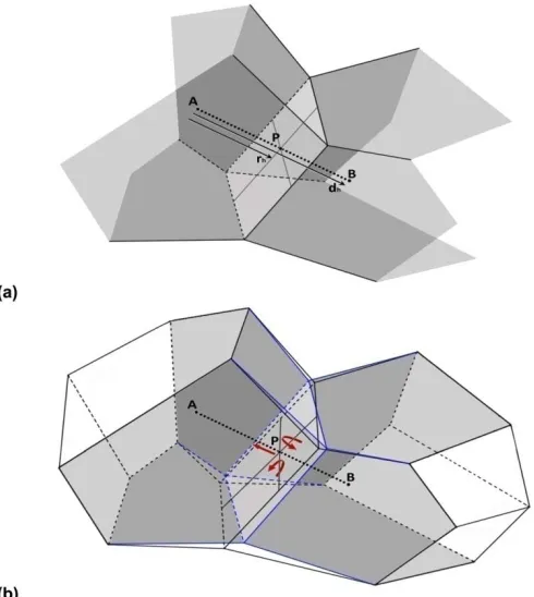
The LT and LVT (Laguerre Voronoi Tessellation) on the contrary, are not evolutionary: they use a non-Poissonian process to position the generators. In particular, the centres are chosen in such a way that spheres with a known size distribution centred on them do not overlap ( (Yang, et al., 2002), (Wu, et al., 2010)). In practice, the LT and LVT increase the degrees of freedom of the VT by placing the interface plane in a position shifted with respect to the midpoint of the segment connecting the neighbouring generators (Figure (1b)). This intersection position, guaranteeing neighbouring spheres not to collide, can be seen as the result of a pseudo growth-rate associated to each centre and expressed under the form of sphere radius ( (Fan, et al., 2004), (Wu, et al., 2010), (Lochmann, et al., 2006)).

Figure II - 1. Resulting microstructures by using (a) VT, (b) LT, (c, d) JMT. The generator

With the idea of a growth rate in mind, the JMT tries to obtain a microstructure by defining a reference cell around each centre and simulating a constant and uniform growth of them. All cells are inflated till they collide and this collision is tracked point by point. Spherical cells are generally used as starting point, resulting in curved cell-cell interfaces. The final geometrical structure is completely unknown ( (Farjas, et al., 2008), (Gilbert, 1962), (Pineda, et al., 2004), (Ferenc, et al., 2007)) and concave cells can be possibly obtained. The big advantage of the JMT lays in its physical basis, as it tries to simulate the actual process of nucleation and growth in order to obtain a realistic microstructure (Figures (1c), (1d)).

2.3.2 Modified Voronoi Tessellation (MVT)

Voronoi Tessellation enforces a dependence of the cell shape on the mutual positioning of the generators: this limits and constrains the possible configurations and topological properties that can be obtained when describing the packed arrangements of objects with a given distribution. To better clarify this point and its implications, let’s consider the simple case of a cluster of randomly arranged spheres (effectively mimicking an aggregate of equiaxed grains) with a lognormal distribution of diameters (see Figure (2a)). Clearly, the Voronoi Tessellation obtained from the centres of the spheres does not match the actual microstructure (see the dashed lines and the shaded area in Figure (2a)). Voronoi Tessellation is in fact unable to randomly pack a given set of unequal spheres: once a (quasi-)spherical shape of the cells is chosen and a given sphere is selected (grey cell in Figure (2b)), the possible size and position of the neighbouring cells is determined. Given a point, the direction where to place a neighbour determines the orientation of a face of the cell (direction and face are orthogonal), whereas the distance fixes the cell size along that direction. To avoid the unphysical resulting superposition (cf. Figure (2b)), the neighbouring objects should then elongate (Figure (2c)). This is an intrinsic limitation of Voronoi Tessellation that goes beyond the sophisticate evolutionary procedures employed e.g. by Gross & Li (Gross, et al., 2002) and by Suzudo and Kaburaki (Suzudo, et al., 2009) to build a microstructure with a given distribution. The impossibility of VT to pack equiaxed objects is also the main reason why any evolutionary method inevitably creates non-spherical cell shapes (see Figure (2c)).

As a matter of fact, any tessellation based on the classical norm (excluding the JMT) would lead, in a real case, to polyhedral grains approximating the spheres and not to true spheres. The microstructure of Figure (2a) is actually compatible with a Laguerre Tessellation with generators in the centres of the spheres; to obtain a Laguerre Tessellation of a given sphere set, first a Random Close Packing of Spheres (RCPS) must be calculated (Fan, et al., 2004). This computationally-intensive step cannot be avoided and is not easily parallelisable.

Voronoi Tessellation (MVT). The main differences between PVT (but also VT in general) and MVT lays in the configuration of the cell-cell interface. In particular, its position along the distance of neighbouring centres (Plane Interface Position, PIP) and its orientation with respect to the plane orthogonal to that vector (Plane Interface Orientation, PIO) are modified. Changing those factors, i.e. going towards a more realistic nucleation/growth process (as in the LT and JMT methods), allows the simulation of realistic microstructures with various statistical distributions of geometrical properties and grain types.

Figure II - 2. (a) Random packing of spheres with a lognormal distribution of diameters. The

centres of the spheres form the dashed Voronoi net. (b) Trying to pack spherical objects around a given (quasi-spherical one (gray). The Voronoi points needed to create the gray object must be centres of intersecting spheres. (c) To avoid intersections, the neighbouring objects have to be deformed.

The release of position and orientation of the plane interface is obtained by introducing two additional factors in the geometric procedure of the VT (cf. Figure (3)): a growth factor (GF) displacing each PIP from the mid-point between two generators and a rotation factor (RF) that changes the associated PIO. The growth factor is obtained as the product of a cell growth factor (CGF) isotropic for the cell, plus a face growth factor (FGF) taking into account a directional dependence of the cell expansion (or contraction). The PIP along the segment connecting two nearest centres A and B is obtained by equilibrating the GF of the corresponding grains, as in: ( ) ( ) ( ) ( ) ( ) ( ) ( ) ( ) ( ) ( ) GF A CGF A FGF AB GF B CGF B FGF BA

GF A PIP d AB

GF A GF B = = = +    (1)

where d(AB) is the distance between A and B.

The cells in MVT are convex polyhedra, but they are usually not space filling: some void regions are created at the cell junctions, as the relaxation of the Voronoi tessellation constraints does not guarantee the compatibility of the geometry of the cells. These voids can be seen as a closed porosity and can form connected networks so counting them has a limited meaning. The presence of the voids is not a serious limitation for the aim of the present work, i.e. the application of the MVT to build a microstructure. Independently of the porosity, the boundary microstructures obtained by filling the cells with atoms are non-physical and need at least a MD equilibration ( (Xu, et al., 2009), (Xu, et al., 2010)). Therefore, as there is no definitive experimental result on the boundary structure (Van Swygenhoven, 2002), several methods can be proposed to take the voids into account or to eliminate them when filling the cells with atoms: some alternatives will be proposed in next section.

Figure II - 3. Neighbouring grains. (a) Traditional Voronoi Tessellation. Poisson-Voronoi

generators A and B and corresponding Voronoi PIP (P). The distance between the generators d(AB) and the distance of the PIP from A (rA) are also shown. (b) Modified Voronoi Tessellation.

The only limitations to the generality of the resulting cell shape are the number of faces and their flatness. The latter restriction can be removed, for example, by roughening the surface of the cells during the microstructure generation (more precisely, when filling the cells with a given crystallographic structure).Sinusoidal functions (Figure (4a)) or additional protruding shapes (Figure (4b)) can be used to roughen the grain–grain interfaces. However, exotic and, more generally unstable local configurations of the atomic arrangement will be relaxed by the equilibration process.

Figure II - 4. Non flat grain-grain interfaces: sinusoidal shape (a), additional stand out shapes

on the surface (b).

2.3.2.1 Relationships between traditional tessellations and the MVT

To frame the MVT in the existing literature, an analogy between tessellation methods and a nucleation/growth process can be used as shown in Figure (5). The combinations of growing rate and nucleation time show several behaviours respect which VT, LT and JMT methods are limiting cases of a more general tessellation procedure, whereas the MVT is the most flexible linear approximation. Moreover, in MVT the directional contribute introduce a third additional factor not possible to involve in the JMT method.

More precisely, a classical PVT is compatible with an instantaneous nucleation of the generators and a uniform growth of the cells whereas the JMT assumes nucleation being time-dependent and growth being uniform. It can be readily seen, in fact, that the GF for the VT are, for instance,

( ) ( )

VT

( ) ( )

( ) ( ) ( ) 2 CGF A CGF B FGF AB FGF BA GF A GF B PIP d AB

= 

⇔  ₌



⇔ =

⇔ =

The VT and JMT, however, are essentially different in the construction of the interfaces, planar in the one case and curved in the other. Owing to its construction, a VT with curved interfaces cannot be obtained, whereas a JMT with planar interfaces is a special case of the MVT.

Laguerre tessellation, on the other hand, has a quite complex GF:

(

)

2 2

2 2

( )

LT ( ), ( ) 1.0

( ) ( )

( ) 1.0

2

A B

A B

GF A

GF A GF B g g

GF A GF B

d AB g g

PIP

⇔ = + −

+ + −

⇔ =

(3)

A suitable combination of nucleation times and growth rates in respect to the nucleation centres distance is in fact necessary as to guarantee the interfaces between neighbouring grains to be planar and shifted and space filling with respect to the VT case.

Figure II - 5. Classification of the various tessellation methods with analogy to nucleation and

growth with planar or curved interface. The MVT diagram approximations of non-planar interfaces are shown by the green lines.

2.3.3 Constrained Modified Voronoi Tessellation (CMVT)

The MVT allows the construction of a model with a target cell volume distribution simply by choosing an appropriate distribution of CGFs (Suzudo, et al., 2009). If necessary, some of the topological properties of the cells can be modified by suitably tuning the model parameters (e.g. the Cell Centre Positions (CCPs)). Unfortunately, a deterministic solution is not yet available to build a microstructure with a desired set of target properties: to this purpose, an evolutional method using Reverse Monte-Carlo (RMC) and genetic algorithms is here presented.

The CMVT analyzes a large collection of models made by the MVT method using different sets of generator parameter values and selects the one that best matches the target configuration. The models are produced by an iterative process involving a key model (i.e. the best model in a subgroup analyzed in the previous iteration step) as starting condition. As in CVT, we minimize here an objective function χ2_{, given by the sum of the squared distances between target and}

current M properties (respectively, Ptarget _{and P}refined_):

2

2 M target refined

k k

k P P 

χ =

∑

The optimization algorithm involves the following basic scheme:

1) Build a starting solution (Key Model, (KM)) and compute its χ2_(KM).

2) Create a set of trial solutions by changing a few generator parameters of the KM. 3) Based on the trial solutions, generate a set of trial patterns and their

corresponding χ2_(i).

4) Replace the KM with the best model among the current one and the new ones. 5) If the χ2 _{is not minimum or is larger than a chosen threshold value, cycle again}

from step (2).

Several statistical and topological properties, e.g. cell size distribution, cell shape isotropy, misorientation and volume fill density can be simultaneously optimized. Some of them, such as e.g. cell size distribution and cell shape isotropy, show little compatibility (it is difficult to create rounded cells with a given distribution, based on a VT) and therefore a careful convergence strategy is needed to avoid local minima and instability of the optimisation process. The solution envisaged here is to employ a modified objective function:

(

)

2 2 M target refined

spread _k wkPk Pk 

χ = χ +

∑

where a set of weights (wk) and an extra penalty (χ2_{spread) are included to take the}

the target properties. The refined cell structure can be used as is, or employed to generate a polycrystalline cluster as assumed here.

For fast computing, both synchronous and asynchronous multithreading were investigated. In the synchronous case, the Key Model is tested and possibly replaced at the end of each iteration step, requiring all threads to be finished and thus breaking the parallelism. In the asynchronous approach each thread works independently, comparing and possibly replacing the Key Model with its own, without waiting for all other threads to end. The latter approach improves the computing performance by eliminating the dead times, but it is usually less efficient as it requires more iterations (see Figure (19)).

2.4 Results and discussion

2.4.1 Atomic density and voids in MVT-derived microstructures

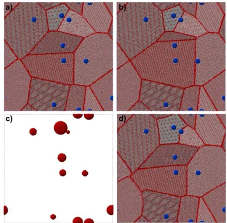
To visually compare the effects induced by different point growth factors on the resulting microstructure, a pseudo-planar case was simulated. A set of centres was produced using a Poisson process with λ= 1 on a square planar region with periodic boundary conditions. Starting from the same set of 14 points, four different microstructures were generated using different MVT setups (see Figure (6)). In Figure (6a), the classical PV Tessellation is shown: the interfaces are halfway between neighbouring points and space filling is guaranteed. In Figure (6b) a lognormal distribution of CGF described as:

( )

exp 2 2 x f x x

µ

σ

σ

π

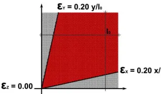
with σ = 0.30, μ = 1.00 was chosen. The shape and size of the domains modifies and a fraction of empty volume is generated in the impingement points of three or more grains. The quantity and the extension of the void regions can be changed by using a more complex set of parameters: in Figure (6c) for instance three different FGF (100 for <1 0 0>, 75 for <1 1 1> and 50 for <0 1 1>; directions referred to the orientation of the local crystallographic reference chosen for each cell) are selected, whereas in Figure (6d) a random perturbation of the interface angles (in the +/- 20.0° range) is applied.

Figure II - 6. Changes in the microstructure caused by a different choice of model parameters.

(a) Voronoi construction, (b) MVT with a lognormal distribution of CGF, μ = 1, σ = 0.30. (c) MVT with different FGF (100 for <1 0 ,0>, 75 for <1 1 1> and 50 for <0 1 1>). (d) MVT with random perturbation of the PIO (limited to +/- 20°). In (e), (f), (g), (h) the detailed construction of a cell with the conditions (a), (b), (c) and (d), respectively. The dashed lines show the modifications occurring to the Voronoi cell in the various cases.

Figure II - 7. Filling of the void resulting from the MVT with (a) empty space (no filling); (b)

amorphous phase (c) crystalline phase and (d) extension of the grains. See text for details.

Voids are filled when the atoms are placed inside the pattern of cells. Four alternatives are here proposed (Figure (7)):

1) leaving voids empty (Figure (7a)): this would effectively simulate a packed aggregate of grains as obtained e.g. in a packed powder;

2) filling voids with a glass phase of given density (Figure (7b)). This would allow a system with completely incoherent grain boundaries to be simulated;

3) filling voids with additional grains possessing independent orientation (Figure (7c)). A fully crystalline structure is obtained, but a possibly unphysical large fraction of very small grains is introduced in the system;

similar to the Johnson-Mehl growing but here a more complex picture of CGF and FGF can be taken into account.

The maximum quantity of atoms that can be placed in the box is not fixed, but depends on factors such as:

• the method used to fill in the cells with the crystallographic structure (for example, a realistic microstructure can be obtained by deleting atoms closer than 85% of the first neighbours distance (Xu, et al., 2009), Figure (8a)); • the way the pattern of cells is built, and the statistical properties of the

microstructure (size distribution, grains number and shape type).

The approach used to fill the grain-grain interface regions entails a strong fluctuation of the quantity of atoms in space: the number is larger for overlapping grain boundary structures (Figure (8b)) than for separate domains (Figure (8c)). Furthermore, the total quantity of atoms in the system can be easily handled by randomly placing atoms in the gap region between separate domains, thus reproducing a liquid phase (Figure (8d)).

Figure II - 8. Cross-section of a Voronoi microstructure. The cells are filled with fcc metal

structure, whereas the grain-grain interface is handled by: eliminating atoms closer than 85% of the shortest neighbour distance (a), and unphysical overlapping of the grain structure for a fixed depth (b), removing atoms at the surface of the cells and leaving separate grains (c), removing atoms at the surface of the cells and filling the so-obtained voids with a liquid phase (d).

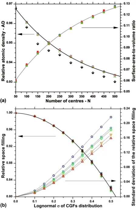
However, independently of all other parameters, the number of grains (i.e. centres) is the key factor to determine the relative atomic density AD (defined as the ratio between the actual atomic density and the maximum one) for a cluster (cf. Figure (9a)). Due to the presence of voids, the atomic density obtained with the MVT is intrinsically lower than that given by the PVT; the difference disappears when the voids are filled using the 4th model (see list above, cf. Figure (9a)).

curves in Figure (9a) can be well reproduced by the two exponentials AD=0.92455+0.05106 exp(N/290.938) and SA/V=0.14626-0.1669 exp(-N/306.434).

Even for a single grain, full atomic density is never obtained in the general case unless box and lattice are suitably chosen (e.g. box scaled with respect to the unit cell and box corners sitting on lattice points).

Figure II - 9. (a) Relative atomic density and surface-area-to-volume ratio versus number of

In any case, nanomaterials cannot be simulated with full atomic density owing to the presence of a large fraction of lower-density grain boundaries where empty volume accumulates. The situation presented in Figure (9a), however, refers only to the geometrical construction: changes are expected when the geometrical microstructure is evolved using, e.g. Molecular Statics or Molecular Dynamics.

The actual values of the input parameters of MVT have a strong effect on the space filling ability. A decrease in space filling ability is usually observed when increasing the dispersion of growth and rotation factors: however, the trend is not monotonous and it is possible to find combinations of parameters which give a better filling of the space. The relative space filling Sf (fraction of volume occupied by the cells in a unity volume inside the box) is independent of the density of centres in the simulation box and decreases steadily for increasing breadth of the input distribution. As an example, Figure (9b) shows the case of a lognormal distribution of CGF with μ = 1. The curve can be well modelled as Sf = 1 – 0.01449 σ – 0.069477 σ2_{. When}

increasing the breadth of the input distribution of CGFs, the distribution of the Sf becomes more symmetrical (the skewness approaches zero) and its standard deviation becomes proportionally larger (see Figure (9b)). It is clear that the higher the σ (i.e. the wider the distribution of sizes), the more difficult is to get a random spatial arrangement of the objects, thus the higher the chances that empty regions (voids) remain (lower space fill). An increase in space filling with respect to Figure (9b) can be obtained by using the CMVT method (Leonardi, et al., 2013).

2.4.2 Statistical properties of the MVT

It is quite interesting to study further the microstructures obtained by MVT when imposing a lognormal distribution of CGF, all other modification parameters being zero (i.e. GF equal to CGF). Figure (10a) shows the average cell volume (V) distributions for the microstructures resulting from the application of the MVT method to the same set of 5000 centres using different lognormal distributions of CGF. The specimens will be identified as MVT x L y where x is the number of centres and y is the σ of the lognormal distribution of CGF (μ = 1.0). Lognormal curve fits are also provided in Figure (10a) as a guide for the eye. For a given distribution of CGF, the result does not modify if the CGF associated to each centre, the μ of the CGF and the box dimensions are changed.

Figure II - 10. Cell volume distribution for a few MVT 5000 samples obtained (a) with different

CGF distributions and (b) with fixed distribution (σ = 0.1) and increasing box size expressed as number of unit cells along the edge: 100 (circle), 150 (square), 200 (diamond), 250 (up triangle), 300 (down triangle). In (c) and (d), respectively, the distributions of total cell surface area and number of faces per cell. The curve proposed by Tanemura (Tanemura, 2003) is shown in (d) as continuous line.

samples made with the same lognormal distribution of CGFs (μ = 1.0 and σ = 0.10) but increasing box size. The independence on box size of the statistical properties allows a coherent scaling of the results obtained on a sample to any other one.

As expected (Figure (10c)) the surface area of the faces and their frequency are almost inversely related. Quite different is the behaviour of NF shown in Figure (10d): all simulated microstructures show exactly the same distribution whose mean (15.5352) is very close to the average facedness of the PVT (2+48π2/35 ≈ 15.53547 ( (Meijering, 1953), (Hilhorst, 2009), (Tanemura, 2003))) and whose shape is compatible with the slightly skewed generalised Gamma distribution proposed by Tanemura (Tanemura, 2003). The agreement comes from the fact that the mutual arrangement, of the centres and thus the average number of near neighbours, is not changed by the MVT. The number of faces of the polyhedral grains, on the other hand, is strictly connected to the geometric construction involved and it is usually close to the number of faces of the dual Voronoi cell construction (10d).

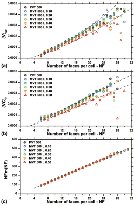
The number of faces is sufficient to characterise several topological properties of the cell. In fact, by using Euler’s formula for convex polyhedron we can relate NF with the number of vertices (NV) and the number of edges (NE) of a cell as NV – NE + NF = 2. The NV can in turn be computed using the equation: NV = 2NF – 4. The changes in NF and in the average volume of the corresponding cell are usually linearly correlated through Lewis’ law (Lewis, 1928): <V>NF = αL (NF - NF0). In the present case, however, a parabolic trend is evident (cf. Figure (11a)): a parabolic violation of Lewis’ law has been already pointed out in both simulated and measured dispersed polycrystalline microstructures ( (Xu, et al., 2009), (Yang, et al., 2002), (Aboav, et al., 1969), (Beck, 1954), (Rivier, 1985)).

The nonlinear trend seems associated to the process employed to lay the centres in the box. In fact, limiting the minimum distance between centres eliminates the nonlinearity: Figure (11b), for instance, shows the modification occurring to Figure (11a) when rising to 20Å the minimum distance between generators. Small deviations from the trends occur at the edges of the NF curve owing to the limited statistics (number of grains) associated to those points. The parameters of the curves slightly change with the increase in the standard deviation of the cell volume distributions, but invariably intercept the axis at NF = 3 (degenerate case). This suggests that the deviation in the slopes of the MVT models is due to the presence of voids, decreasing the cell volume especially of the larger cells. The influence of the voids decreases with the cell size and the axis intercept agree with the impossibility to define a closed polyhedron with less than 4 faces.

A final check for the properties of the cell ensemble is provided by the ratio between the average number of faces in all neighbouring cells to a cell of NF faces (m(NF)) and the number of faces per cell. The relationship is well described by the Aboav-Weaire law (Chiu, 1995):

2

( )

where α and μ are fitting parameters. Mathematically, it expresses the tendency for any random tessellation to have small grains surrounded by large ones and vice

versa.

Figure II - 11. (a) and (b) Lewis plots for the MVT 5000 samples of Figure 6a. The plot in (b)

was obtained by limiting the minimum distance between centres to 20Å. In (c) the Aboav-Weaire plot is shown for the MVT 5000 samples of Figure 6a. Fits are proposed for the limiting cases MVT5000 L 0.1 and MVT 5000 L 0.5.

start with a similar random arrangement of points and that the MVT does not heavily modify the number of faces of Voronoi cells (cf. Figure (10)). A small downward curvature in Figure (11c) seems to be present, confirming the observation of Hilhorst (Hilhorst, 2009), thus strengthening the idea that the Aboav-Weaire law might be just a good local approximation for the correct trend. In the range shown, the modified curve proposed in (Hilhorst, 2009) i.e. NF m(NF) = 8 NF+23.15 NF5/6-15.96 NF2/3 does not appreciably depart from Eq. (7).

2.4.3 Relationship between input parameters and resulting microstructure

A systematic relationship exists between the input CGF distribution and the resulting cell size distribution. It should be stressed that different choices can lead to completely different resulting distributions. For the sake of brevity, just the lognormal case is analysed in detail. Without losing in generality, a collection of samples was simulated with increasing number of centres and different lognormal CGF distributions with lognormal mean μ = 1. A cubic box with PBCs and a side of 100 unit cells was employed. The same naming convention for the samples proposed before will be used here.

Figure II - 12. Mean (a) and standard deviation (b) of the normalised cell volume distributions

as a function of the normalised CGF (where V is the volume of the cells having a reference CGF). Data relative to the MVT5000 L 0.10 (circle), MVT5000 L 0.20 (square), MVT5000 L 0.3 (diamond), MVT5000 L 0.4 (down triangle), and MVT5000 L 0.50 (up triangle).

general) expresses the fact that if the centres would be isolated, their size at a given time would be proportional to their growth rate. The standard deviation for each CGF value, on the other hand, is related to the magnitude of the difference between isolated growth and actual growth (constrained by the interference with the other centres). Therefore, the growth rate represents somehow the probability of interference between neighbouring centres. In particular, centres with a small growth rate (small CGF) interfere with the neighbouring centres after a longer time than those with a higher growth rate (high CGF).

The PVT method is the simplest case of constant-rate growth. Therefore, the cell size distribution of a PVT reflects exactly the distribution of the half distances of the neighbouring centres. In a sample created by the PVT method, the cell radius computed from the cell volume and from the mean plane interfaces distance show exactly the same distribution and almost the same values. A change in the size distribution is strictly connected to any change of the arrangement of the centres. For instance, the CVT method drives the centres towards a configuration where the distribution of plane interface distances is comparable with the target cell volume distribution. As previously noted, this leads to non spherical cells; in particular, cells with the largest standard deviation are more anisotropic (Xu, et al., 2009). Removing the constraints imposed by the Voronoi construction, allows moving the centres independently of the cell shape: a full control over anisotropy (and therefore roundness of the cells) is thus possible.

Figure II - 13. Relationship between the σ of the input lognormal distribution of CGF and the

Figure (13) shows a clear parabolic relation between σ of the CGF (σin) and

both μ and σ of the corresponding cell volume distribution. Independent of the

number of centres, the two parabolas can be parameterised as μ = -0.0674 – 2.0149 σ in (13a) and σ = 0.4454 + 2.2455 σ in (13b). The result is

compatible with the PVT where σ = 0.445 is obtained when fitting the resulting distribution with a lognormal (Meijering, 1953). The data spread around the best fit in Figure (13) can be related to the statistics of the corresponding distributions. The picture does not change if the size of the box, the number of centres and the μ of the lognormal CGF distribution are changed. The behaviour shows significant deviations if the homogeneous Poisson point process with parameter λ=1 is not used. A characteristic relation is observed when imposing a minimum distance between neighbouring cell generator centres: the higher the threshold value of the neighbour distance, the smaller the variances of the log-normal best fit cell volume distributions (see Figure (14)). The possibility of having the same cell statistical and topological properties, by varying only one or simultaneously more than one generator parameters, support the unconstrained nature of MVT. Actually, compared with homogeneous Poisson, slightly lower significance values are found for the agreement between cell volume and log-normal distributions.

Figure II - 14. Relation between σ of the input lognormal distribution of CGF and the resulting σ

of the best fit lognormal output distribution of V/<V> for specimens of increasing shortest distance between generator centres. Shortest distances are expressed as fraction of the minimum neighbour distance for the density equivalent fcc structure: 1/3 (up triangle), 1/4 (down triangle), 1/6 (diamond), 1/12 (square), and Poisson point process (circle).

the trend of the CSD versus the σ of the input distribution of CGF. The average cell surface density decreases with increasing distribution width. The trend is similar independently of the number of centres, but the actual values steadily increase with the increasing quantity of generators. An increase of the standard deviations of CGF distribution causes a general decrease of the global surface of the cells: in fact, the larger the spread of the cell sizes, the smaller the volumetric contribution of smaller cells for a constant box volume. It is well know that in a box of constant volume a system of smaller spheres would have a larger surface than a system of large ones. For a given distribution, moreover, an increase in the number of centres causes a decrease of the mean cell size, and therefore a corresponding increase in the cell surface density, as experimentally observed.

Figure II - 15. Dependence of the cell surface density versus the σ of the input CGF for an

increasing number of centres (1000: up triangle, 2000: down triangle, 3000: diamond, 4000: square, 5000: circle).

2.4.4 Reliability of MVT statistics by the evolutionary CMVT

All evolutionary processes were started here with a cubic box having Periodical Boundary Conditions (PBCs). A thousand centres were placed in the box by a homogeneous Poisson point process with λ=1 and were assigned suitable CGF values. The initial CGFs were chosen according to a Log-normal Probability Density Function (PDF) with unit mean:

2

2

1 ln

exp 2 2

Log normal

x PDF

x

µ σ πσ

−

 _{ − }  = −_ _ 

 

 

(8)

a similar way as in (Leonardi, et al., 2012(d)), samples are here named CMVT x L y I z, where x is the number of centres, y is the starting σinput of the

Log-normal PDF of the input CGFs, and z is the number of iterations. It has been already shown in (Leonardi, et al., 2012(d)) that null FGFs and PIOs lead to a normalised cell volume PDF being close to the expected Log-normal. In that case, the standard deviation of the Log-normal frequency distributions of the target normalised cell volume (σexpected) and of the input CGF (σinput) are quadratically

dependent and σexpected=0.4454+2.2455 σ2input (Leonardi, et al., 2012(d)).

Three cases were simulated here: CMVT 1000 L 0.10, 0.20 and 0.30. Significant sample populations were defined for each one of those cases, repeating 100 times the evolutionary process with different random initial configurations. The starting average levels of significance over the population with respect to the expected PDF (σ = 0.4679, 0.5352 and 0.6475) were, respectively, 23.01%, 35.34% and 38.74%. The levels of significance computed via Kolmogorov-Smirnov (KS) hypothesis test were improved by the constrained algorithm. The initial configurations were evolved by varying each starting CGF by a random factor 0.10 < δ < +0.10, without changing any other generator parameter.

Figure II - 16. (a) mean and standard deviation of the levels of significance of the CMVT 1000 L

0.10, 0.20 and 0.30 I 1000 populations during the evolutionary processes; the results for a single run of CMVT 1000 L 0.10, 0.20 and 0.30 I 10000 is also provided to confirm the observed trend (in this case the standard deviations are not available). (b) distributions of significance levels of CMVT 1000 L 0.30 after 10, 100, and 1000 iteration steps.

smaller the average variances (Figure (16a)). When increasing the number of iterations, the distribution of the levels of significance tends to become more left-skewed (Figure (16b)). Hence, a target level of significance can generally be reached by varying just the CGF values, without changing the generators (as in the CVT method).

The normalized cell volume distributions of the evolved samples (averaged over each of the three populations) are in good agreement with the target PDFs, as computed by the KS hypothesis test (cf. Figure (17a)). The evolutionary process has significantly changed the absolute values of the CGFs, raised from 1.0 to 2.8 in 1000 iterations. Nevertheless, the normalized CGF distributions of the evolved samples are very close to the initial ones. The average frequencies over each of the three populations show Log-normal PDFs (see Figure (17b)). The standard deviations of the Log-normal best fit of the CGF distributions of CMVT 1000 L 0.10, 0.20 and 0.30 I 1000 are close to the input values (respectively: 0.1363, 0.2165 and 0.3104).

Figure II - 17. Normalized cell volume (a) and CGF (b) frequency distributions of CMVT 1000 L

0.10, 0.20 and 0.30 I 1000.

2.4.5 Multiple target properties optimization with CMVT

Differently from the CVT, the CMVT method is able to yield several independent pattern configurations with similar statistical and topological properties by combining more than one generator parameter (e.g. CGFs and CCPs). This greater flexibility allows the CMVT method to optimize at the same time more than one statistical and topological property of the model.

cell size distribution, maximum volume fill density and cell shape isotropy. Since a generic collection of spheres cannot tessellate the space, volume fill density and spherical shape turn out to be incoherent. The equiaxed shape has been thus chosen as target property and the standard deviation of the distance between cell faces and generator centres was minimised.

Figure II - 18. Improvement history of the properties for the evolutional process about CMVT

1000 L 0.10 (a limit number of 100000 iterations was imposed).

Figure II - 19. Improvement ratio for synchronous (dark continuum line) and asynchronous

The convergence efficiency was improved by assigning a higher weight to the equiaxial character (double with respect to the others). In this case, the new models created at each iteration step are obtained by randomly changing both the generator centres (two in the box and two near the corresponding positions of the KM) and the CGF (by a random factor 0.10 < δ < +0.10). Figure (18) shows the percent improvement of each property P, defined as (Pcurrent-Pinitial)/(Ptarget-Pinitial)%, during the

evolutional process: the improvement is logarithmic, with convergence speed increasing stepwise with the iteration number. Synchronous and asynchronous multithreading approaches were employed. Despite the larger collection of models investigated by the second approach, the improvement ratio seems strictly dependent on the number of iterations (see Figure (19)).

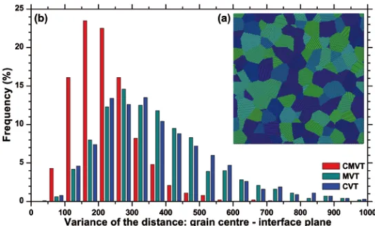
Once the pattern with the required properties is obtained, the atomistic microstructure can be built. In each cell, the generator and the centres of mass are more or less coincident. A planar section (Figure (20a)) shows features that cannot be obtained by other tessellation methods: for instance, the grain-grain interfaces are not placed in the middle between the generator centres as in the case of the VT method, and the topological properties of the cells are not directly correlated with the cell size distribution. This can be also appreciated in Figure (20b), presenting the distributions of the variances of the distances between grain centres and grain interface planes of both the CMVT 1000 L 0.10 I 100000 and two other models having the same cell size distribution, but made by CVT and MVT.

Figure II - 20. (a) Plane section of CMVT 1000 L 0.10 I 100000 polycrystalline microstructure.

(b) Frequency distribution of the variance of the distances between grain centres and grain interface planes.

deviation (μ ≈ 225, σ ≈ 92). Still, an ideal value for the sphericity (Ψ) defined on the basis of the surface and volume of the cells (S and V, respectively) as:

[

]

3

6V S

π π

Ψ = (9)

cannot be achieved by any VT or MVT pattern, being each cell a convex polyhedron. Since a generic collection of spheres cannot tessellate the space, volume fill density and sphericity turn out to be incoherent. Notwithstanding, a significant improvement of the sphericity is still found in the CMVT simulation (see Figure (21)).

Figure II - 21. Frequency distribution of the sphericity for CMVT 1000 L 0.10 I 100000. The two

extreme shapes for the given cluster are shown as a reference. 2.4.6 MVT computing performance

We have shown that the MVT can directly provide a microstructure with a given size distribution variance and with a shape close to lognormal. Unlike the VT, however, computing time for the MVT is not linearly related to the number of centres, but it depends on the actual properties of the input distribution. This is a consequence of simultaneously dealing with all centres and corresponding growth factors to compute the shape of the resulting cell, while keeping full record of the voids.

broader the distribution, the larger the fraction of void space (cf. Figure (9b)), thus the longer time and the larger memory for recording information about intersection of interface planes.

Figure II - 22. Time required by the MVT method to compute the microstructure (i.e. to identify

the faces of all cells) for the MVT 1000 set of specimens.

2.5 Conclusion

A Modified Voronoi Tessellation (MVT) has been proposed to simulate a realistic microstructure. To obtain that, MVT starts with a random distribution of centres in a box (with or without periodic boundary conditions) and builds the corresponding cells by relaxing the Voronoi constraints on the cell-cell interfaces, i.e. by shifting and rotating them with respect to the midpoint between neighbouring centres. The resulting microstructure (pattern) is characterised by the presence of voids that can be easily eliminated when filling the cells with atoms. A one-to-one relationship between the input model parameters and the characteristics of the output distribution has been found, allowing a target distribution to be directly obtained. For instance a lognormal distribution of grain sizes can be directly simulated with a 5% level of significance. The statistical correlation between the Log-normal distribution of the Cell Growth Factors (CGFs) and the Log-normal cell sizes distribution of a pattern made by the MVT method was confirmed and extended by the Constrained MVT.

The Constrained Modified Voronoi Tessellation method (CMVT) is also proposed to generate polycrystalline microstructures characterized by more than one target statistical and topological property. Space fill density, size distribution and isotropic cell shape are optimized by varying the generator parameters (Cell Centre Positions and Cell Growth Factors): a logarithmic improvement is obtained through an evolutional approach. Thus, realistic microstructures can be obtained beyond the limits imposed by the traditional tessellation techniques.

Chapter III

Analysis of Atomistic Simulation Data

Part of this chapter has been published in:

Alberto Leonardi, Kenneth Roy Beyerline, Tao Xu, Mo Li, Matteo Leoni, Paolo Scardi

“Microstrain in nanocrystalline samples from atomistic simulation”,

Zeitschrift für Kristallographie Proceeding, I (2011) 37-42.

Alberto Leonardi, Matteo Leoni, Mo Li, Paolo Scardi

“Strain in atomistic models of nanocrystalline clusters”,

Journal of Nanoscience and Nanotechnology, (2012) accepted.

3.1

Abstract

Atomistic modelling was employed to investigate the effect of microstrain on X-ray diffraction patterns in nano-crystal microstructures. Stress and a strain defined on atomic scale from atom positions were computed to represent the local deformation associated with the microstructure (e.g. grain boundaries).

Strain, as an easy and clearly defined concept in continuum mechanics, has no direct counterpart in atomistic models. Existing methods, relying on the concept of atomic coordination number, do not provide a complete description of isotropic and anisotropic strains across metallic nano-crystalline microstructures. To overcome those limitations a new method is proposed: the Voronoi Cell deformation (VCD) fully accounts for the local geometry and provides a description of the strain field independent of the atomic coordination.

3.2

Introduction

Atomistic simulation is recognised as a reliable tool to investigate the structure and properties of nano-scale materials as it can provide atomic-level picture along with the macroscopic collective behaviour comparable to experimental results. This is particularly valuable in the field of nano-structured materials where the microstructures can be created using space filling models ( (Gross, et al., 2002), (Suzudo, et al., 2009)) and then simulated by Molecular Dynamics (MD).

Atomistic modelling is increasingly employed to study properties and behaviour of materials under different conditions (Derlet, et al., 2005). Although results do not always match those of traditional experiments, this approach is informative and can most frequently capture the main features of the physical phenomena of interest ( (Jang, et al., 2006), (Cao, 2009), (Van Swygenhoven, et al., 2000), (Li, et al., 2006)). The limited extension of the time scale commonly accessible to MD simulations penalizes some applications, like those concerning plasticity, but is perfectly adequate to represent thermal and elastic properties.

A major task is extracting models of behaviour compatible both with the macroscopic observation and with the MD scale. Most of the relevant literature in the field employs methods utilizing stress, pressure or level of coordination ( (Samaras, et al., 2003), (Zimmerman, et al., 2004), (Derlet, et al., 2005)) while strain is seldom used (Stukowski, et al., 2009). For certain theoretical analysis, this is sufficient since direct extraction of strain from the stress is not easy. However, the methods based on stress or pressures are not of general applicability to a given sample as they rely on the knowledge of atomic velocity or interatomic potential. Strain, however, is not properly defined at the atomic level because the traditional definition, based on continuum mechanics, does not apply to discrete systems on the atomic level. The complexity is even larger if atomic vibrations are to be considered as well.

Among the available methods, Neighbours Analysis (NA) studies the local geometrical arrangement of neighbours to detect structural features at the atomic level ( (Ackland, et al., 2006), (Honeycutt, et al., 1987)). NA is a powerful tool to identify defects and phases in large systems, but is intrinsically unable to provide strain values. Therefore, NA is complemented by methods to calculate local pressure and stress ( (Samaras, et al., 2003), (Derlet, et al., 2003), (Derlet, et al., 2006)), as those properties are directly related to the energy of each atom, with no need to define or calculate strains.

coordinated. To overcome this limitation we propose the Voronoi Cell Deformation (VCD) method. Based on Voronoi Tessellation, the VCD avoids the somehow arbitrary concept of cut-off radius, required by existing methods ( (Stukowski, et al., 2009), (Lewis, 1928)). Moreover, as it makes no reference to the atomic coordination, the VCD can be used across heavily defected regions as well as in the core of nano-structured domains.

Furthermore, from the dynamics, or time evolution of the atoms trajectories, we can compute the mean square displacements which contribute directly to the line broadening in the powder diffraction patterns. As a result, we are able to compare, on a continuum scale, the characteristics of the calculated strain distribution and the microstrain obtained from a traditional X-ray diffraction (XRD) Line Profile Analysis (LPA).The line profile broadening in an XRD pattern is affected by the distribution of strains at the atomic level (microstrain) inside a material. Microstrain can be analyzed by traditional and modern line profile analysis methods: a correct evaluation in nano-crystalline materials is however difficult due to the peculiar m