Nonlinearities
A
process is said to be linear if the process response is proportional to the stimulus given to it. For example, if you double the amount deposited in a conventional savings account (the stimulus), then you will receive double the interest (the response). Similarly, if you work ten percent longer hours, you would hope to accomplish ten percent more work. These are linear responses.Models that assume a process is linear have been extensively studied because the mathematics for such models is relatively straightforward, and linear models can adequately represent the behavior of many realistic processes over a useful range of conditions. It is often possible to solve the equations for linear models without the need to use computers. Thus, in the era before the widespread availability of computers, the ease of solution for linear models led to their use even in situation where the real-world process was known to benonlinear.
Many business processes are nonlinear, especially when pressed to extremes. For example, while it may be true that if you work ten percent longer hours you will accomplish ten percent more work, it is probably not true that if you work twice as many hours you will accomplish twice as much work. Many of us have attempted to do this, and have soon su±ered from \burnout" leading to a reduction in our working e±ectiveness. This is a nonlinear response. Similarly, the available production capacity may limit the amount of a product that can be sold, regardless of the amount of sales e±ort or the degree of customer demand. In other cases, such as graduated income taxes or variable interest rates on money market accounts, nonlinear responses are deliberately designed into the system. With graduated income taxes, the amount of tax grows more rapidly than the increase in income, and with a money market account the rate of interest may grow more than proportionally as the balance grows.
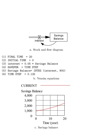
Figure 8.1 shows the stock and ¯ow diagram, Vensim equations, and a graph of Savings Balance for a conventional savings account with compound interest where the interest is left to accumulate in the account for 20 years. The interest rate is ve percent (0.05) per year, and the initial balance is $900. After 20 years, the balance has grown to a little over $2,400. The response (that is, the earned interest) is linearly related to the initial amount placed in the account.
Using IF THEN ELSE to Model Nonlinear Responses
Some money market accounts have a sliding interest rate where the interest rate depends on the balance in the account. For example, suppose that an interest rate of ve percent (0.05) per year is paid on every dollar in the account up to $1,000, and an interest rate of ten percent (0.10) per year is paid on every dollar in the account over $1,000. Then the interest is given by
interest =
8 < :
0:05¡ Savings Balance; Savings Balance<$1;000 0:05¡ 1;000
+0:10¡ (Savings Balance 1;000); otherwise
A somewhat generalized version of this model is shown in Figure 8.2. In Figure 8.2, the Savings Balance amount at which the interest rate changes is speci ed by the constant BREAKPOINT (which is 1,000 for this example), the interest rate paid on each dollar below BREAKPOINT is speci ed by the con-stant LOW RATE (which is 0.05), and the interest rate paid on each dollar above BREAKPOINT is speci ed by the constant HIGH RATE (which is 0.10). (The use of these constants, rather than \hard wiring" in speci c values for BREAK-POINT, LOW RATE, and HIGH RATE, facilitates sensitivity analysis using the automated features of Vensim. This is discussed further below.)
From Figure 8.2c, we see that the Savings Balance after 20 years is over $3,400, which is substantially more than with the conventional savings account shown in Figure 8.1. (Note that the increase in savings rate for most real-world money market savings accounts above the BREAKPOINT is usually not as great as shown in this example! The large value used in this example for HIGH RATE makes it easier to see the impact of the nonlinear interest rate.) A detailed examination of the model output shows that the Savings Balance exceeds the BREAKPOINT value of $1,000 during the second year, and after that the money market account generates more interest than the conventional savings account.
interest
Savings Balance
a. Stock and ¯ow diagram
(1) FINAL TIME = 20
(2) INITIAL TIME = 0
(3) interest = 0.05 * Savings Balance
(4) SAVEPER = TIME STEP
(5) Savings Balance= INTEG (interest, 900)
(6) TIME STEP = 0.125
b. Vensim equations
CURRENT
Savings Balance
4,000
3,000
2,000
1,000
0
0
10
20
Time (year)
c. Savings balance
HIGH RATE LOW RATE
BREAKPOINT
interest
Savings Balance
a. Stock and¯ow diagram
(01) BREAKPOINT = 1000
(02) FINAL TIME = 20
(03) HIGH RATE = 0.1
(04) INITIAL TIME = 0
(05) interest=
IF THEN ELSE(Savings Balance < BREAKPOINT, LOW RATE * Savings Balance,
LOW RATE * BREAKPOINT
+ HIGH RATE * (Savings Balance - BREAKPOINT)) (06) LOW RATE = 0.05
(07) SAVEPER = TIME STEP
(08) Savings Balance= INTEG (interest, 900)
(09) TIME STEP = 0.125
b. Vensim equations
CURRENT
Savings Balance
4,000
3,000
2,000
1,000
0
0
10
20
Time (year)
c. Savings balance
HIGH RATE from the beginning, while this does not happen with the interest for the Initial Balance of $900 speci ed in Figure 8.2 until the Savings Balance reaches $1,000.
The IF THEN ELSE feature illustrated in equation (05) of Figure 8.2b pro-vides a powerful and¯exible way to model this type of nonlinear response. For example, it is possible to nest a second IF THEN ELSE within the rst one to handle a situation where there is a second breakpoint at which the interest rate earned on each dollar changes again.
Using Lookup Functions to Model Nonlinear Responses
In addition to the IF THEN ELSE function, another approach to modeling nonlinear responses is provided by many simulation languages using \lookup functions." A Vensim model for the money market account example which uses a lookup function is shown in Figure 8.3. With this approach, the nonlinear response function (which is \interest" for this example) is modeled by entering several pairs of points. The simulation program then creates a curve through these points which is used to determine the necessary values to run the simula-tion.
Equation (4) of Figure 8.3b de nes this lookup function, which is called IN-TEREST LOOKUP. This function is speci ed by the three pairs of points (0, 0), (1000, 50), and (2000, 150). These points specify that there is $0 of interest per year earned on a Savings Balance of $0, $50 of interest earned per year on a Savings Balance of $1,000, and $150 of interest earned per year on a Savings Balance of $2,000. In Vensim, the lookup function calculates intermediate val-ues by drawing straight lines between the speci ed pairs of valval-ues. Thus, the complete lookup function is shown in Figure 8.3c.
A casual examination of the Figure 8.2 and Figure 8.3 models indicates that these are the same, and thus they should show the same Savings Balance. How-ever, a comparison of Figure 8.2c with Figure 8.3d shows that the Savings Bal-ance curves are somewhat di±erent. What has happened?
The di±erence between the curves shown in Figure 8.2 and Figure 8.3 illus-trates a potential di° culty with using lookup functions. The lookup function in equation (4) of Figure 8.3b is speci ed over a range of values for Savings Balance from $0 to $2,000. However, the actual Savings Balance exceeds $2,000 during the thirteenth year. The speci ed behavior for a lookup function in Ven-sim when the range is exceeded is to \clamp" the output of the function at the highest speci ed value. Thus, whenever the Savings Balance is above $2,000, the lookup function INTEREST LOOKUP gives an output of $150. Clearly, this is incorrect for this savings account! (Vensim generates a warning message whenever the range speci ed for a lookup function is exceeded. In this particular case the following message is generated: WARNING: At 13,25 Above
``INTER-EST LOOKUP'' computing ``interest.'')
INTEREST LOOKUP interest
Savings Balance
a. Stock and ¯ow diagram
(1) FINAL TIME = 20
(2) INITIAL TIME = 0
(3) interest = INTEREST LOOKUP(Savings Balance)
(4) INTEREST LOOKUP([(0,0)-(2000,200)],(0,0),(1000,50),(2000,150))
(5) SAVEPER = TIME STEP
(6) Savings Balance= INTEG (interest, 900)
(7) TIME STEP = 0.125
b. Vensim equations
CURRENT
INTEREST LOOKUP
200
150
100
50
0
0
1000
2000
-X-CURRENT
Savings Balance
4,000
3,000
2,000
1,000
0
0
10
20
Time (year)
c. Lookup function d. Savings balance
(4) INTEREST LOOKUP([(0,0)-(5000,500)],(0,0), (1000,50),(5000,450))
which expands the upper limit for the range of INTEREST LOOKUP from a Savings Balance of $3,000 up to $5,000. When this change is made, identical output is generated to that shown in Figure 8.2c.
Comparison of IF THEN ELSE and Lookup Functions
The IF THEN ELSE and lookup functions each have advantages and disadvan-tages for modeling nonlinear functions. As Figure 8.2b shows, it is possible to include constants in an IF THEN ELSE function so that a sensitivity analysis can be conducted directly in terms of the model constants BREAKPOINT, LOW RATE, and HIGH RATE using the automated procedures in Vensim. This can-not be done so directly when a lookup function is used. (Vensim does support a sensitivity analysis feature where a lookup function can be temporarily changed for a particular model run, but some calculation is necessary to determine ex-actly how the lookup function points must be changed to represent particular low and high interest rates for the money market account model.)
On the other hand, a lookup function can easily be constructed for situations where there are more than one breakpoint. While this can be done with IF THEN ELSE functions by nesting them, this can lead to complex function expressions.
8.2 Resource Constraints
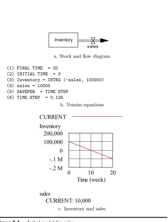
Another common cause of nonlinear responses in a business process is resource constraints, such as limits on available personnel or production capacity. Figure 8.4 illustrates a rst attempt at a model for a simple situation of this type where there is a xed Inventory of 100,000 units available to sell, and a sales rate of 10,000 units per week. As the curves in Figure 8.4c demonstrate, this rst model is inadequate. The Inventory drops to zero at ten weeks, but sales continue undiminished at a rate of 10,000 units per week. While an order backlog might grow for a while when the product is not available, sales are likely to drop as customers cannot get the product. The constraint on the number of units available to sell needs to be included in the model.
sales Inventory
a. Stock and¯ow diagram
(1) FINAL TIME = 20
(2) INITIAL TIME = 0
(3) Inventory = INTEG (-sales, 100000) (4) sales = 10000
(5) SAVEPER = TIME STEP
(6) TIME STEP = 0.125
b. Vensim equations
CURRENT
Inventory
200,000
100,000
0
-.1 M
-.2 M
0
10
20
Time (week)
sales
CURRENT: 10,000
c. Inventory and sales
sales Inventory
a. Stock and ¯ow diagram
(1) FINAL TIME = 20
(2) INITIAL TIME = 0
(3) Inventory = INTEG (-sales, 100000)
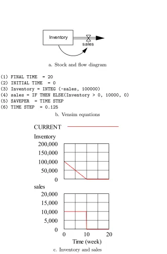
(4) sales = IF THEN ELSE(Inventory > 0, 10000, 0)
(5) SAVEPER = TIME STEP
(6) TIME STEP = 0.125
b. Vensim equations
CURRENT
Inventory
200,000
150,000
100,000
50,000
0
sales
20,000
15,000
10,000
5,000
0
0
10
20
Time (week)
c. Inventory and sales