Structure and properties of nanostructured materials from atomistic modeling and advanced diffraction methods

(1)

Structure and properties of nanostructured

materials from atomistic modeling and

advanced diffraction methods

Luca Gelisio

(2)

Approved by

Prof. P. Scardi, University of Trento

Prof. I.K. Robinson, London Centre for Nanotechnology Dr. P. Frontera, Mediterranean University of Reggio Calabria

(3)

(4)

Contents

List of Equations vi

List of Algorithms vii

List of Tables vii

List of Figures vii

1 Introduction 1

2 Atomistic simulations 3

2.1 Interaction potential . . . 4

2.1.1 Adiabatic approximation . . . 5

2.2 Classical molecular dynamics . . . 6

2.2.1 Molecular dynamics algorithm . . . 7

2.2.2 Microstates and macrostates . . . 8

2.2.3 The bulk-like system . . . 9

2.2.4 Remarks on the choice of the potential . . . 10

2.3 Analysis of results . . . 10

2.3.1 Atomistic deformation . . . 11

2.3.2 Radial pair correlation function . . . 13

2.3.3 Mean squared displacement . . . 13

3 Atomistic approach to scattering 15 3.1 Intensity scattered by an atomic aggregate. . . 17

3.2 Powder average of the intensity . . . 19

3.2.1 Computational aspects. . . 21

(5)

Contents

3.3.1 Coherence and correlation . . . 24

3.3.2 Uncorrelated crystallites . . . 30

3.4 Demonstration of the paradigm . . . 35

3.5 Assumptions . . . 39

4 Small crystallites 40 4.1 Crystallite response to surface tension . . . 42

4.1.1 Effect of surface relaxation on powder patterns . 42 4.1.2 Models for surface relaxation . . . 44

4.1.3 Shape-effect on deformation . . . 50

4.2 Atomic vibrations . . . 51

4.3 Modeling the pattern from metal nanocrystals. . . 55

4.3.1 Whole powder pattern modeling . . . 56

4.3.2 Challenging interpretation paradigms . . . 57

4.4 Conclusions and outlook . . . 68

5 Modeling scattering data 69 5.1 The modeling engine . . . 69

5.1.1 Parameters . . . 71

5.1.2 Programming . . . 72

5.1.3 Alternative engines . . . 72

5.2 Truncated palladium nanocubes. . . 73

5.2.1 Atomistic model . . . 74

5.2.2 Morphological dispersion . . . 75

5.2.3 Powder diffraction pattern. . . 78

5.2.4 The sample . . . 84

5.3 Conclusions and outlook . . . 86

6 Outlook 88

Abbreviations 91

Symbols 93

(6)

List of Equations

2.2 Hamiltonian operator for an atomic aggregate . . . 5

2.3 Schrödinger equation . . . 5

2.7 Thermal de Broglie wavelength . . . 6

2.8 Newton’s second law of motion . . . 6

2.9 Ergodic hypothesis . . . 8

2.10 Time average . . . 9

2.12 Average-position configuration. . . 11

2.20 Radial pair correlation function . . . 13

2.21 Average number of nearest neighbors . . . 13

2.22 Radial pair correlation function and structure function . 13 2.23 Mean square displacement . . . 14

2.24 B-factor . . . 14

3.1 Wavevector transfer . . . 16

3.3 Atomic form factor . . . 16

3.4 Spherical approximation to the atomic form factor . . . 17

3.5 Structure factor . . . 17

3.6 Intensity distribution . . . 18

3.9 Debye scattering equation . . . 20

3.17 Debye scattering equation for interference effects . . . . 30

4.1 Young-Laplace equation for a spherical object . . . 44

4.2 Radial strain at the particle/vacuum interface . . . 45

4.3 Ishikawa model for surface relaxation. . . 46

4.4 Beyerlein model for surface relaxation . . . 47

4.5 Huang model for surface relaxation . . . 47

4.6 Atomistic deformation due to surface tension . . . 48

4.8 Young’s modulus along directionˆr . . . 50

5.1 χ2_{for a given configuration} _{. . . .} ₆₉

(7)

5.9 Pseudo-Voigt function . . . 80

5.10 Chebyshev polynomials of the first kind . . . 81

5.14 Transmittance of impinging intensity . . . 83

5.15 Transmittance of a beam on a cylindrical sample . . . . 83

List of Algorithms

2.1 Simplified molecular dynamics algorithm . . . 7

5.1 Outline of the simulated annealing algorithm . . . 71

List of Tables

2.1 Thermodynamic ensembles . . . 8

3.1 GPU technical details . . . 23

4.1 Physical properties of Rh, Pd, Ag, Pt and Pb . . . 58

5.1 Palladium physical properties . . . 77

5.2 Parameters varied during data modeling . . . 86

(8)

List of Figures

3.3 Small crystal showing stacking faults . . . 18

3.4 Spherical average of vectorrmn . . . 19

3.5 The Debye scattering equation . . . 20

3.6 Evolution of GPU computing power in recent years . . . 22

3.7 Rotating atomic aggregate and ensemble equivalence . . 25

3.8 Effect of misorientation on intensity distribution . . . . 27

3.9 Simplified model to investigate correlation . . . 29

3.10 Self- and cross-correlation . . . 31

3.11 Correlation parameter . . . 33

3.12 Correlation within a realistic microstructure . . . 34

3.13 Graphite oxide dispersed in water. . . 36

3.14 Powder pattern of a graphene layer . . . 36

3.15 Disordering a graphite cluster . . . 37

3.16 Pattern of a disordered graphite cluster . . . 38

4.1 Small slab of aluminum placed on top of a nickel substrate 41 4.2 Radial strain for a spherical copper aggregate . . . 45

4.3 Debye scattering equation applied to a spherical copper aggregate . . . 46

4.4 Radial strain for a spherical copper aggregate computed along selected directions . . . 48

4.5 Strain field across a palladium cube . . . 49

4.6 Symmetry of palladium Young’s modulus . . . 51

4.7 Effect of aggregate shape on atomic displacement . . . . 52

4.8 Average strain as a function of aggregate shape . . . 53

4.9 Average Biso as a function of aggregate shape . . . 54

4.10 Average MSD as a function of the radial position . . . . 55

4.11 WPPM for spherical aggregates . . . 59

4.12 WPPM view of the relative change of unit cell . . . 60

4.13 Biso as a function of elastic properties . . . 61

4.14 Biso as a function of the considered element . . . 62

4.15 WPPM view of the TDS . . . 63

4.16 WPPM view of micro- and macrostrain . . . 64

4.17 Warren’s diagram considering an anisotropic RMSD model 65 4.18 DSE modeling of surface relaxation effects . . . 67

5.1 Tuning parameters . . . 72

(9)

List of Figures

5.3 Fingerprint smoothing by morphological dispersion . . . 76 5.4 Powder diffraction sphere intersecting the {200}

(10)

Chapter 1

Introduction

Matter at thenanoscaleexhibits peculiar properties, often not shown by the bulk counterpart, and strongly coupled to the specific size, shape and structure of the atomic aggregate. Particularly, the enormous surface-to-volume ratio implies boosted reactivity with respect to the environment, while the electronic confinement might cause quantum effects to dominate physical properties.

One famous experiment demonstrating the size-dependency of the melting temperature of gold was given by Buffat and Borel [1], which re-ported this quantity to vary from the bulk value, approximately 1300K, to 800K for an aggregate as small as 2.5nm diameter. By the way, pe-culiar properties revealed at the nanoscale have been exploited since thousands of years, exempli gratia the Lycurgus Cup [2], adiatretum belonging to the 4th century AD, dichroic because of optical properties of gold-silver nanostructured particles embedded in the glass matrix. Nature also exploits nanotechonology, employed for example to cre-ate diffraction gratings on the wings of some butterflies or to produce self-cleaning lotus leafs.

The range of applicability of nanostructured materials is enormous, with notable cases in catalysis and medical imaging.

(11)

temporal resolution. In a different realm, atomistic simulationshave also greatly evolved deriving advantages from both recent theories and modern computing units. In this framework, a detailed description of the system in a spatial and temporal range compatible with lengths probed by scattering techniques is provided.

In a single sentence, the subject of this Thesis is the effort of tying atomistic methods and scattering techniques so to increase the compre-hension around size, shape and structure of nanostructured particles.

(12)

Chapter 2

Atomistic simulations

If, in some cataclysm, all of scientific knowledge were to be destroyed, and only one sentence passed on to the next gen-eration of creatures, what statement would contain the most information in the fewest words? I believe it is the atomic hy-pothesis (or the atomic fact, or whatever you wish to call it) that all things are made of atoms – little particles that move around in perpetual motion, attracting each other when they are a little distance apart, but repelling upon being squeezed into one another. In that one sentence, you will see, there is an enormous amount of information about the world, if just a little imagination and thinking are applied.

R.P. Feynman, 1964 [3]

(13)

2.1. Interaction potential

Computer experiments are chiefly a tool to predict/understand the properties of materials. If experimental conditions are precisely mim-icked, simulation results can be, more or less directly, compared with observed data. This allows the underlying theoretical model to be tested and, in case it is accurate, the simulation can assist in the in-terpretation of results. On the other hand, any arbitrarily difficult – or impossible – condition to be measured can be thought and realized. For instance, properties of iron at the pressure and temperature of Earth’s core can be determined [10].

Broadly speaking, MMC methods consist in stochastically generat-ing a set of atomic positions accordgenerat-ing to an appropriate statistical-mechanical distribution, therefore granting access to static equilibrium averages (see e.g. [11]). Dynamic properties are available from MD simulations, a deterministic technique where the time evolution of a many-body system is described by solving the Newton’s equations of motion [12] (see section2.2).

While producing a comprehensive theoretical framework for atomistic simulations is beyond the scope of this document, some selected con-cepts and methods concisely follow-up. Superb reference sources are, in my opinion, the evergreen by Allen and Tildesley [13], books by Frenkel and Smit [11] and by Leach [14] and the document by Erco-lessi [15]. The formalism used to connect microscopic and macroscopic realms is the one of statistical-mechanics, thoroughly explained, for example, in the book by Chandler [16] or the one by Tuckerman [17].

2.1

Interaction potential

Atomic interactions are of course ruled by quantum mechanics. The full non-relativistic Hamiltonian for an atomic aggregate is

ˆ

H= ˆK+ ˆV = ˆKn+ ˆKe+ ˆVnn+ ˆVne+ ˆVee, (2.1)

(14)

2.1. Interaction potential

electrons, equation2.1can be expressed (using atomic units) as

ˆ H= N ∑ n=1 ˆ p2 n 2mn

+ E ∑ e=1 ˆ p2 e 2m′_e +

1 2 N ∑ n=1 N ∑ u=1

ZnZu ∥rn−ru∥

+1 2 E ∑ e=1 E ∑ l=1 1 ∥r′_e₋_r′_l∥ −

N ∑ n=1 E ∑ e=1 Zn ∥rn−r′e∥

,

(2.2)

where m,p,ˆ Z andrare, respectively, the mass, the momentum oper-ator, theatomic numberand theposition vectorof a nucleus whereas primed quantities refer to an electron. The solution of the Schrödinger equation [18],

ˆ

HΨ(r,r′) =EΨ(r,r′) (2.3) provides the total wave function (rand r′ are, respectively, the set of all nuclear and all electronic coordinates) and therefore the complete description of the system.

2.1.1 Adiabatic approximation

To reduce the complexity of the problem, Born and Oppenheimer in-troduced the adiabatic approximation [19], built around the concept that electrons move faster than nuclei (being much lightweight) and adiabatically follow nuclear motion. Electronic and nuclear motion are therefore separated in this framework and the wave function, in turn, is expressed as

Ψ(r,r′) =ψN(r)ψE(r′;r), (2.4) being ψN and ψE the wave function of the nucleus and of the elec-tron (which parametrically depends on nuclear positions), respectively. Equation2.3can therefore be divided into an electronic equation (con-sidering fixed nuclei positions),

( _E ∑ e=1 ˆ p2 e 2me

+1 2 N ∑ n=1 N ∑ u=1

ZnZu ∥rn−ru∥

+1 2 E ∑ e=1 E ∑ l=1 1 ∥r′_e₋_r′_l∥

− N ∑ n=1 E ∑ e=1 Zn ∥rn−r′e∥

)

ψE(r′;r) =V (r)ψE(r′;r),

(15)

2.2. Classical molecular dynamics

and a nuclear equation,

( _N

∑

n=1 ˆ p2

n 2mn

+V(r) )

ψN(r) =E ψN(r), (2.6)

where the quantity V (r) is the interatomic potential. Further step, if the paradigm is the classical molecular dynamics, the Schrödinger equation can be replaced by Newton equation.

2.2

Classical molecular dynamics

The evaluation of the thermal de Broglie wavelength [20],

Λ= √

2πℏ2 mkBT

(2.7)

being m the atomic mass, T the temperature of the system, ℏ the reduced Planck constant and kB the Boltzmann constant, permits to discriminate between quantum and classical regime. Particularly, if that wavelength is smaller than the mean nearest neighbor separation (Λ ≪ a), then the classical approximation is justified. For instance, the thermal de Broglie wavelength of a crystal of palladium atoms (m = 106.42amu) at room temperature (T = 273.15K) is Λ ≈ 0.1Å, much smaller than the lattice parameter (a = 3.890Å), therefore le-gitimizing nuclei to be considered as classical particles. In general, quantum effects tend to be relevant for lightest atoms and/or cold-est temperature. In fact, if equation 2.7 is applied to helium atoms (m = 4.002602amu) at T = 4K, then Λ ≈ 4.4Å, too wide to neglect quantum effects.

If the adiabatic approximation holds, the time evolution of a set of in-teracting atoms (a many-body system) is obtained in the framework of classical molecular dynamics from the numerical solution of Newton’s equations of motion, which conserve the total energy of the system E=K+V. The force acting on atom nis calculated as

(16)

2.2.1 Molecular dynamics algorithm

The starting point of aMDsimulation is the generation of a plausible atomic structurerand velocity fieldr, typically drawn from a Maxwell-˙ Boltzmann distribution [21,22] at a given temperature. An interatomic potential V(r) is then specified, together with a timestep δt for the numerical integration of equations of motion. The step is a crucial parameter to be selected since, if too small computer time is wasted, otherwise numerical instabilities arise causing the energy conservation and time-reversibility to fail. Therefore, as a general rule the timestep should be a couple of orders smaller than the reciprocal of the highest-frequency motion,i.e. usually of the order of 1fs.

Before iterating, it is often opportune to minimize the energy of the initial configuration, therefore migrating to a nearby local minimum of the potential energy surface.

TheMDloop proceeds until the desired time te is reached, evolving from the starting configuration through an equilibration phaseto the production phase, during which properties are calculated. At every iteration forces are computed according to equation 2.8whereas veloc-ities and positions are obtained integrating according to some finite difference method,e.g. the velocity Verlet algorithm [23], depicted at line 6in algorithm5.1.

Algorithm 2.1 Simplified molecular dynamics algorithm conserving total energy and implementing the velocity Verlet integrator.

1: r(t= 0),r˙(t= 0),V (r)andδt

2: (energy-minimize configuration)

3: Fn(t= 0) =−∇rnV (r(t= 0))

4: whilet < tedo

5: Fn(ti+1) =−∇rnV (r(ti+1))

6:

{ ˙

rn(ti+1) =r˙n(ti) + [Fn(ti+1) +Fn(ti)]δt/2m rn(ti+1) =rn(ti)δt+Fn(ti) (δt)

2 /2m

7: ti←ti+δt

(17)

2.2.2 Microstates and macrostates

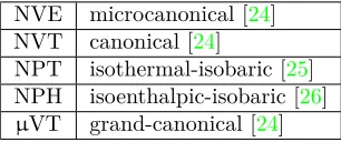
AMD simulation results in a temporal sequence of 3N positions and 3N momenta, i.e. a trajectory. This is naturally described in the 6N-dimensionalphase space, each point corresponding to amicrostate, i.e. a configuration of the system. The collection of points in phase space satisfying the constrains of a particular thermodynamic state (macrostate) is an ensemble, which is said to be in statistical equilib-riumif it does not evolve over time. The most natural thermodynamic ensemble forMD, i.e. the one obtained from the solution of equation 2.8 and discussed so far, is themicrocanonical ensemble (NVE) char-acterized by the number of atoms N, the volume of the systemV and the total energyEto be fixed to a given value. Other thermodynamic ensembles are reported in table2.1.

NVE microcanonical [24] NVT canonical [24]

NPT isothermal-isobaric [25] NPH isoenthalpic-isobaric [26]

µVT grand-canonical [24]

Table 2.1: Thermodynamic ensembles. The acronym in the first column is constructed from corresponding fixed variables. N is thenumber of atoms,

Vthevolume,Ethetotal energy,Tthetemperature,Pthepressure,H the enthalpy andµthe chemical potential.

The connection between microstates and macrostates (the thermody-namic observables) is operated by the tools of statistical mechanics. Experimentally accessible quantities are generally obtained by prob-ing a huge number of atoms samplprob-ing many microstates and therefore the macroscopic behavior of the system can be calculated by averaging over the ensemble, i.e. by integrating over the phase space of the sys-tem. If the ergodic hypothesis [27] holds, then the system will evolve through all possible microstates over asufficient period of timeand the ensemble average will equal the time average,

Ao=⟨A (Γ(t))⟩e =⟨A(Γ(t))⟩t (2.9)

(18)

over the ensemble (e) or over time (t). The time average is constructed in the conventional way,

Ao=⟨A(Γ(t))⟩t= lim

τ→+∞ 1 τ

∫ τ

t=0

A (Γ(t′))dt′≈ 1 S

S ∑

t=0

A (Γt).

(2.10) being S the number of steps in the simulation.

2.2.3 The bulk-like system

It is often desirable to investigated properties of abulk system which, in principle, should contain an infinite number of atoms and no sur-faces. While this condition is rather unpractical to achieve in a MD simulation, nevertheless it can be mimicked implementing theperiodic boundary conditions (PBCs)[28]. For simplicity, consider a simulation box (but the reasoning can be extended to other geometries [14]) de-scribed by edges{Li, Lj, Lk} replicated an infinite number of times to describe a periodic lattice completely filling space. The coordinates of then-th atom in thei-thimage cell are expressed by the relation

r(i)

n =rn+aiLiˆi+ajLjˆj+akLkkˆ ai, aj, ak ∈Z (2.11) whereˆ_i,ˆ_j_and_kˆ _{are unit vectors codirectional with coordinate system.} As an atom exits the original cell, one of its periodic images enters from an adjacent cell therefore conserving the number of elements.

Care must be taken when implementing thePBCssince some artifacts are introduced. The first intuitive consideration is that the size of the cell should exceed the interaction distance of the interatomic potential so that atomn does not interact with its own image. If this condition is not satisfied the symmetry of the cell is imposed on the system [13]. Secondly, the characteristic length of the investigated property should be smaller than the size of the cell since the maximum wavelength of the density waves (fluctuations) is related to the latter quantity. Low-frequency phonons and shock waves are affected, for example, and displacement fields can interact.

(19)

2.3. Analysis of results

2.2.4 Remarks on the choice of the potential

The realism of a simulation extremely relies on the choice of the poten-tial. Many alternatives exist, commencing with the simple Lennard-Jones (pair) potential [29], still employed because of its computational efficiency. When dealing with metals, a widely employed formalism is the embedded atom method (EAM) [30–33] or its modified version (MEAM) [34]. Within the class of bond order potentials, thereactive force field (ReaxFF)[35–38] permits bonds to be formed and broken, therefore allowing chemical reaction to take place. Next level of com-plexity, the electron force field eFF [39,40], is a semiclassical approach which allows dealing with excited systems by representing electrons as Gaussian wave packets and nuclei as point charges.

Many more models for the interatomic potential exist, characterized by a different degree of accuracy and computational complexity. The choice of the optimal potential depends on the specific tackled problem (chemical composition and bonding, size and time scale, ...) and on the kind of information to be extracted (structural, chemical, ...).

To conclude, the size- and time-scale which can be simulated are con-tinuously increasing, both because of the uninterrupted growth of com-puting power, both because of advances in methodology.

Of particular interest is the so-calledmultiscale modeling, which com-bines techniques characterized by different levels of accuracy (e.g., quantum, atomistic, mesoscopic and continuum), each solving a spe-cific part of the problem (seee.g. [41–44] and references therein).

2.3

Analysis of results

• ◦ • ◦ •Part of this section has been adapted from [45–47].

(20)

Configuration

The configuration is the set of the positions r forming a body. The starting guess of the system, constructed according to some mathe-matical recipe, is called as-built configuration.

Thetime-averaged configurationof the quantityA (r(t))has already been defined (⟨A (r(t))⟩tin equation2.10), whereas theaverage-position

configuration is expressed as

Ap=A (⟨r(t)⟩t). (2.12)

As will be shown, this quantity permits to remove dynamical features (atomic vibrations) so to single out the static displacement field.

2.3.1 Atomistic deformation

Deformationis the transformation from a reference configurationr0to

the present, deformed configuration rd (see e.g. [48]). The change in configuration results in an atomic displacement,

u=rd−r0, (2.13)

independent of the choice of the reference frame and defining a field. This quantity is in general composed by (i) a rigid-body displacement (translation/rotation), preserving distances between atoms; (ii) a defor-mation, defined by a nonzero relative displacement between particles and therefore changing the shape and/or size of the body.

An immediate visual perception of the deviation from the reference configuration is offered by the displacement, which hereinafter is con-sidered to be relative, free from any rigid-body motion. To treat e.g. surfaces, it is useful to extract the component of the atomic displace-ment projected on the plane described by the normalp,ˆ

P⊥

ˆ

p (un)=un−(un·pˆ)pˆ (2.14) and normal to the plane,

(21)

so that P⊥

ˆ

p (un)+Ppˆ(u)= un. Alternatively, the displacement can be projected onto a given vector like the case ofcoherent X-ray diffrac-tion (CXD)imaging [49–51],Q·un, whereQis thewavevector transfer (scattering vector)which will be introduced in chapter3.

To get rid of any physical dimension the concept ofstrain, the normal-ized relative displacement, is also introduced. Because of deformation, atomic volume can be modified: a simple method to measure atomic volume is by calculating the Voronoi tessellation [52] of the atoms.

The average atomistic strain can be evaluated by computing the dif-ference ofbond length(the Euclidean norm ofrnm=rn−rm,nbeing a nearest neighbor ofm) and averaging the information over thenumber of nearest neighbors(N),

bn= 1

Nn

Nn ∑

m=1

∥rnm∥. (2.16)

The average strain of atomic bonds of a given atom n as seen by its nearest neighbors can therefore be expressed as

εb,n= bd b0

−1. (2.17)

To provide a “surface view” of the above quantity,Nn nearest neigh-bors are identified by drawing an annulus centered on the given atom in thereference (as-built) configuration, with mean radius equal to the first neighbors distance, and lying on the plane described by the nor-mal versorp. The neighbor list computed in the previous step is thenˆ used to draw the vector connecting atoms n and m in the deformed configuration and the strain is again evaluated according to equation 2.17, representing in this case the average strain of a given atomn as seen by its nearest neighbors lying on the plane described by p.ˆ

Different views of the strain can be built considering the symmetry of the atomic aggregate. For example, theradial strain

εr,n= un·ˆrcn

∥rcn∥, (2.18)

(22)

2.3.2 Radial pair correlation function

The average number of atomic pairs separated by a distancerat time t is given by

p(r, t) = 1

N N ∑ n=1 N ∑ m=1 m̸=n

δ(∥rnm(t)∥ −r), (2.19)

beingδ(x)the Dirac-delta function [53], which is practically computed by compiling a histogram of separations within each interval r+Δr. For an isotropic and homogeneous system having numeral density ρ, theradial pair correlation function (RPCF)is defined as (seee.g. [13,

16,54, 55] for a more rigorous definition)

g(r)= 1 ρN ⟨ _N ∑ n=1 N ∑ m=1 m̸=n

δ(∥rnm(t)∥ −r) ⟩

e

. (2.20)

Since the number of particles within the spherical shell of radiirandr+ dris4πr2g(r), the integration over the region of theRPCFextending from r₋ tor+, provides an estimate of theaverage number of nearest neighbors,

N = 4π

∫ r+

r=r₋

g(r′)r′2dr′. (2.21)

Interestingly, the RPCFis related to an experimental accessible quan-tity, thestructure functionS(Q), through a Fourier transform. Assum-ing an isotropic sample (apowder, described in section3.2) composed of a unique chemical species [56–58],

g(r)= 1 + 1 2π2_r_ρ

∫ _∞

Q=0

Q′[S(Q′)−1]sin(Q′r)dQ′, (2.22)

where Qis the modulus of the wavevector transfer (scattering vector).

2.3.3 Mean squared displacement

(23)

rfrom a reference configuration, which can be either theas-builtr0or

theaverage-position ⟨r(t)⟩t, like in this case,

⟨u(t)2⟩= 1

N

N ∑

n=1

∥rn(t)−⟨r(t)⟩tn∥2. (2.23)

In other words, if dealing with the solid state of matter this quantity express the mean square amplitude of atomic oscillations. TheMSDis in turn related to the (isotropic)B-factor, which appears in the Debye-Waller temperature factor [59, 60], by the time average of the MSD,

Biso= 8π2

3 ⟨⟨u(t) 2

⟩⟩t. (2.24)

(24)

Chapter 3

Atomistic approach to scattering

The physical principles of the interaction between X-rays and matter are discussed in many books. Among them, in my opinion, two must-readsare the one by Guinier [61] and the one by Warren [57]. Although they are not the most up-to-date references (original versions date back to, respectively, 1956 and 1968), nevertheless they gracefully provide an astonishing multitude of concepts essential to understand X-ray scattering. A sublime contemporary source introducing X-ray physics and covering a broad set of techniques is the book by Als-Nielsen and McMorrow [62]. The main goal of this book is to present developments in X-ray science after the introduction of synchrotron radiation sources, in the late seventies.

(25)

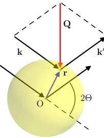
being thewavevector transfer (scattering vector)

Q=k−k′. (3.1)

If the scattering event is elastic, then ∥k∥ =∥k′∥ and thereforeQ= ∥Q∥= 2∥k∥sinΘ= (4π/λ)sinΘ.

O

k0

k

r Q

2Θ

Figure 3.1: An X-ray impinging with wavevectork on the charge element of an isolated atom at positionris elastically scattered tok′. Geometrical definition of the wavevector transfer (Q) and of the scattering angle (2Θ) is also shown.

The integration of the contribution of each volume element to the scattered field engender the definition of theatomic form factor,

f0(Q)=

∫ _∞

0

ρ(r)exp(ıQ·r)d3_r

=FQ[ρ(r)] (Q), (3.2)

i.e. the Fourier transform of the charge density. By virtue of the quantum mechanics nature of electrons, theatomic form factoractually depend on the energy of the incoming beam,

†_f_(Q_,_ℏ_ω₎₌_f0₍_Q_{) +}_f′₍_ℏ_ω_{) +}_ı_f′′₍_ℏ_ω₎_, _(3.3)

where f′ and f′′ are the dispersion corrections tof0. Often inX-ray diffraction (XRD) data interpretation spherical symmetry is invoked

(26)

3.1. Intensity scattered by an atomic aggregate

to simplify the non resonant term (equation 3.2) off(Q,ℏω), which can then be expanded as [65]

f0(Q)=

4 ∑

i=0 aiexp

( −bi

[

Q

4π

]2)

+c (3.4)

Theory and tables for atomic form factors can be found e.g. in [62,

64–66] and analogous quantities exist for the interaction of neutrons and electrons with matter.

3.1

Intensity scattered by an atomic aggregate

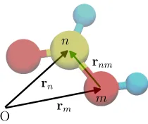
Extending the reasoning carried out for the isolated atom to an atomic aggregate (molecule) composed ofN atoms,e.g. the one in figure3.2, thestructure factorcan be expressed as

F(Q)= N ∑

n=1

fn(Q)exp(ıQ·rn), (3.5)

being the nucleus of the n-th atom connected to the reference frame by the vector rn andfn its form factor.

O rn

rm

rnm

n

m

Figure 3.2: Formic acid molecule. Nucleus of the carbon atom (yellow) is connected to the origin of the reference frame (O) by vectorrn.

(27)

3.1. Intensity scattered by an atomic aggregate

However, last step can be avoided and the atomic aggregate considered to be a single molecule rather than a tiny crystal [67]. The quantity effectively probed during an experiment is the intensity distribution (figure3.3),i.e. thestructure factortimes its complex conjugate

I(Q)=F(Q)F∗(Q)

= N ∑

n=1

fn(Q)exp(ıQ·rn) N ∑

m=1

f_m∗ (Q)exp(−ıQ·rm)

= N ∑

n=1 N ∑

m=1

fn(Q)fm∗ (Q)exp(ıQ·rnm),

(3.6)

being rnm=rn−rm,i.e. the vector connecting atomsnandm.

Figure 3.3: Portion of a small palladium spherical crystal showing a de-formation and a twin fault. Purple arrow coincide with the (111) direction and yellow cylinders are drawn to guide the eye. Red, Green and Blue indi-cate, respectively, position of layers A, B and C (left). Intensity distribution (isosurfaces) around(111)RSpoint calculated from equation3.6(right).

(28)

3.2. Powder average of the intensity

3.2

Powder average of the intensity

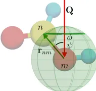
• ◦ • ◦ •Part of this section has been adapted from [47,68,69]. Let the molecule sketched in figure 3.4 rotate with respect to the in-coming beam, taking every possible orientation with equal probability. Relative atomic positions are fixed and the motion is rapid enough that only the average scattered intensity is observed.

rnm

n

m ψ φ Q

Figure 3.4: The head of the (green) vector connecting atommton (rmn) takes with equal probability every possible orientation with respect to the wavevector transfer (Q) drawing the green spherical surface. Polar (ψ) and azimuthal angle (ϕ) are also indicated.

During its motion, the head of the vector rnm spawns the spherical surface in figure3.4. Mathematically, the powder average of the inten-sity distribution is expressed by the orientational (spherical) average of equation3.6(assuming spherically symmetricatomic form factor),

⟨I(Q)⟩o= N ∑

n=1 N ∑

m=1

fn(Q)fm∗ (Q)⟨exp(ıQ·rnm)⟩o. (3.7)

The result of the spherical average of the exponential term in the equa-tion above,

⟨exp(ıQ·rnm)⟩o=

∫ 2π

ϕ=0

∫ π

ψ=0

exp(ıQrnmcosψ)r2nmsinψdϕdψ

∫ 2π

ϕ=0

∫ π

ψ=0

r2

nmsinψdϕdψ

(29)

leads to the definition of theDebye scattering equation (DSE), derived for the first time by Debye in 1915 [70],

I(Q)= N ∑ n=1 N ∑ m=1

fn(Q)fm∗ (Q)sinc(Q rnm). (3.9)

Therefore, the powder average of the intensity distribution depends only on the magnitude of the interatomic distances (rnm) and not on their mutual orientations.

-60 -30 0 30 60

rx, ˚A

-60 -30 0 30 60 ry , ˚ A

2 4 6 8 10

Q, ˚A−1 0.0 0.5 1.0 1.5 2.0 2.5 3.0 in tensit y / N 2f 2 0(Q

=

0)

10−4

10−2 ₁₀−1 ₁₀0

10−6

10−5

10−4

10−3

10−2

1010−1 0

−4 −2 0 2 4 Qx, ˚A−1

−4 −2 0 2 4 Qy , ˚ A − 1

Figure 3.5: The DSE (red) applied to a palladium Marks decahedron (bottom, left), normalized over the squared number of electrons, i.e.

N2f02(Q= 0). Small angle region of the pattern is reported in the inset

(30)

TheRSview of the procedure used to deduce theDSElies in a (spher-ical) surface integral (powder diffraction sphere, depicted in figure3.5) of theintensity distribution. Traditionally, this procedure is simplified by the tangent plane approximation [71] invoking the argument that intensity distribution is concentrated around RS points (seee.g. [47] and references therein).

3.2.1 Computational aspects

One of the major limitations to a broad application of theDSEhas been its computational requirements. Indeed, the number of calculations for a given value of wavevector transfer equals the squared number of atoms.

Several methods have been proposed to mitigate computational require-ments. In the pioneering work of Germer and White (1941) on elec-tron diffraction [72], the pattern for a powder of particles made of 55 atoms was obtained by manual calculations, exploiting crystal symme-try. Particularly, they recasted theDSEfor a monoatomicfcccrystal as

I(x)= pairs_∑

n=0

Bnf2(x)sinc

(

x√n), (3.10)

x=π√2Ra0/Lλbeing a function of the electron wavelength (λ), unit-cell parameter (a0) and other experiment-dependent features (Lis the specimen-plate distance,Rthe abscissa of the microphotometer curve). The termBn is twice the number of atom pairs having the separation a0√n/2in the crystal, withB0=N. Germer and White accomplished to compute the DSEof even larger particles (up to 379 atoms, which corresponds to a spherical copper crystal described by a diameter of 20.4Å) by introducing the approximation, for large values ofN,Bn=

Nbnϵn. The term bn =a0 √

n/2 is the number of atoms at a given distance in an infinite fcc crystal and ϵn, which lies in the range 0≤ ϵn ≤1, accounts for the shape of the crystal.

(31)

containingp(rk)values, leading to the following variant of theDSE

I(Q)=f2(Q) bins ∑

k=1

p(rk)sinc(Q rk). (3.11)

A further step forward was the adoption of a fast Fourier transform (FFT) algorithm in place of the explicit summation, as proposed by Hall and Monot in 1991 [74], elegantly improved by Cervellino and colleagues who proposed a clever method to obtain a continuous distri-bution function of distances by smoothing theRPCFwith a Gaussian function. This function is then re-sampled with a constant step, so that the FFT can be efficiently used to generate the powder pattern. The Gaussian smoothing can be easily removed via multiplication by an inverse function.

2006 2007 2008 2009 2010 2011 2012 2013 2014 1

2 3 4 5 6

Theoretical

FLOPS,

10

12

8800

280

480580 680

Titan Black Titan

Figure 3.6: Theoretical single-precision (black dot) and double-precision (gray dot) peak performances (FLOPS) of some NVIDIA® _{GeForce GTX}

(32)

The tremendous computational power ofGPUshas been exploited to allow the application of the original formulation of the DSE[68, 69]: the embarrassingly parallel nature of equation 3.9 perfectly fits the data-parallel vocation ofGPUs. No approximation (apart from those inherent in the use of floating point math) is therefore enforced and the DSEcan be safely applied to any type of atomic aggregate. The theoretical number of FLOPS of modern graphics cards, reported by figure3.6for some selected devices, outperform the throughput of cen-tral processing units (CPUs) and the growth rate of their computing power in the last half decade is impressive. To be included in the list of advantages, the modest power consumption (and relatively low price) ofGPUsallows multiple devices to be hosted by a single desktop com-puter. Some technical details of processing units hosted by the personal computer used to calculate patterns presented in this chapter are re-ported in table3.1. Although thetheoretical number ofFLOPSis just a rough indicator of computing power of processing units, nevertheless it offers a fair indication of achievable performances.

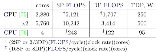
cores SPFLOPS DPFLOPS TDP, W GPU[75] 2,880 †5,121 †1,707 250

x2 5,760 10,242 3,414 500

CPU[76] 4 ‡243 ‡122 95

†_{(2SP or 2/3DP)(}_FLOPS_{/cycle)(clock rate)(cores)} ‡_{(16SP or 8DP)(}_FLOPS_{/cycle)(clock rate)(cores)}

Table 3.1: Technical details of the central (Intel® _{Core™ i7-2600K) and}

graphics (2 NVIDIA® _{GeForce GTX TITAN Black) processing units on the}

desktop computer used to calculate diffraction patterns presented in this chapter. Quantities shown here are the number of theoreticalFLOPSwhen performing single precision (SP) and double precision (DP) operations. The thermal design power (TDP), a conventional figure used to express the ther-mal load generated by a given device and therefore proportional to the peak power consumption, is also reported.

(33)

3.3. Interference in a scattering experiment

3.3

Interference in a scattering experiment

The methods of Debye [70] are accepted in the scattering of electrons by gases, but despite the application to thin films by Germer and White [72] their use in kinematic electron diffraction from polycrystalline solids has seemed suspect and none of the recent texts on electron diffraction mention the methods. [...] The objection to the Debye theory is that it neglects interference between atoms situated in different crystals; while this is permissible for a gas of large molecules, it requires justification if the molecules (or small crystals) are densely packed.

C.W.B. Grigson, 1967 [78]

• ◦ • ◦ •Part of this section has been adapted from [45].

In section3.2, theDSEhas been derived envisaging a particlerotating so to take every possible orientation with equal probability. Yet, this condition would be difficult to encounter in a real scattering experi-ment. Imagine notwithstanding a large ensemble of copies of the very same atomic aggregate randomly directed and arranged in space, as the one depicted in figure 3.7. If it was possible that the elements of the collection scatter independently, without any kind ofinterference, then it can be demonstrated that the signal scattered by the ensem-ble exactly equals the output of the DSE applied to a single element multiplied by the number of items in the collection. This important result, which strictly speaking only applies if copies are separated by an infinite length, guarantees equation 3.9 to be applied to real case studies.

3.3.1 Coherence and correlation

Interference among scattering domains causes specific features to ap-pear[79–84], which modify the traditional concept of crystallite. As shown by Rafaja and colleagues [79,80,82,83], those effects are clearly visible when (i) the scattering domains are sufficiently small and (ii) strongly textured. Effects of interference were observed in nanocrys-talline thin films deposited by physical vapor deposition (PVD) [80,82,

(34)

The general understanding of this effect is that whenintensity distribu-tionfrom different crystallites overlap inRS, the observed line profiles tend to sharpen, the peak width being related to a larger size than that of the single domains. Effects tend to be observed more at low diffraction angle, corresponding to RSpoints closer to the origin.

Figure 3.7: On the right, a large ensemble of copies of the atomic aggregate drawn on the left, randomly oriented and arranged, separated by an infinite distance.

Interference in a scattering experiment results either from properties (i) of the beam (coherence) and (ii) of the sample (correlation). An interesting discussion on their interplay is given in [85] and [86].

3.3.1.1 Coherence

(35)

3.3.1.2 Correlation

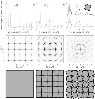
The correlation lengths are related to inhomogeneity of the specimen (size and defects) and define the concept ofcrystallite,i.e. a coherently scattering domain (where scattered waves are in phase). In the simpli-fied model of ideally imperfect crystal, ormosaic, first introduced by Darwin in 1922 [87], a real crystal is though of as if composed of many perfect-crystal blocks, slightly misoriented with respect to each other. Interference only occurs inside each block (crystallite), whose size there-fore defines the correlation length, and not among waves diffracted from different domains. Thus, the scattered intensity from the whole mo-saic equals the sum of intensities diffracted by each block (at least in the wide angle region if the correlation volume is infinite, as it will be assumed to be hereinafter) as it is demonstrated in figure3.8c.

Imagine partitioning the perfectly crystalline cubic domain depicted in figure3.8a in blocks (grains) and then rotating them by a given angle about a randomly oriented axis. If the misalignment is sufficiently large and random, as in figure 3.8c, then each grain in the polycrystalline aggregate will scatter incoherently, as in the mosaic model and the width of each diffraction peak (and in turn, the correlation length) will be related to the average size of the block. Indeed, as demonstrated by the powder diffraction pattern in figure 3.8c, the diffracted intensity from the whole mosaic equals the sum of the intensities scattered by each grain when considered as an isolated object.

The other extreme behavior is observed when blocks are not misaligned at all, and they will obviously scatter coherently and the width of the diffraction peak will be related to the size of a larger object, the cubic domain itself illustrated by figure 3.8a.

Intermediate misalignments, as shown in figure 3.8b, cause intensity scattered from different blocks to overlap inRSin such a way that the concept of crystallite becomes apparently dependent on the magnitude of the wavector transfer modulus.

(36)

(37)

Effect of rotation From a phenomenological point of view, the effect of rotation is summarized by figure 3.8which leads to three intuitive considerations.

First of all, the probability of intensity overlapping inRS is propor-tional to the size of its distribution and therefore to the inverse of the crystallite size. The smaller the grain, the higher the probability of in-tensity overlapping, and thus the stronger the effect on the scattering pattern. For the sake of discussion, above argument can be expressed considering the Scherrer equation [88,89], expressed inRSas,

ΔQ≈2π

D, (3.12)

where, roughly, ΔQis the broadening of the intensity distribution due to finite size of a sphere of diameter D.

Secondly, rotating two lattices in direct-space (DS)implies the rota-tion of their corresponding reciprocal lattices around a common center, theRS origin. Therefore, the smaller the angleθ between crystallites, the higher the overlapping probability. The last consideration is useful to understand how the effect of misorientation affects scattered inten-sity as a function of the momentum transfer Q.

Lastly, for a given misorientation degree, the overlapping volume be-comes smaller by moving away from theRSorigin since the arc lengths (actually, the great-circle distance on the surface of a sphere) of equiv-alent points belonging to different reciprocal lattices increases linearly with the momentum transfer,

s=θQ. (3.13)

To keep the discussion simple, assume that the arc length can be ap-proximate by the chord d. Then, the common volume between two spherical distributions of intensities of diameter ΔQis,

Ω(ΔQ, d) = π

12(2ΔQ+d) (ΔQ−d) 2

d≤ΔQ, (3.14)

and, after substituting equation3.12and equation3.13,

Ω(D, θ,Q)≈ π 12

( 4π

D +θQ ) (

2π D −θQ

)2

θQ≤2π

D, (3.15)

(38)

Effect of displacement To understand the effect of displacement on correlation it is better to recast thestructure factor. Suppose that the atomn, placed atrn, belongs to grain p, connected to the (global) reference frame by the vector Rp. Then, the position of n in the (local) reference frame anchored to the centroid ofpcan be expressed as rpn=rn−Rp, as sketched in figure3.9. This relation leads to the following definition of the structure factor(see equation3.5),

F(Q)= M ∑

p=1

exp(ıQ·Rp) Np ∑

n=1

fn(Q)exp(ıQ·rn), (3.16)

where the innermost sum accounts for the internal structure of each grain, containing Np atoms, and the outermost one spans the number of grains in the aggregate. The system sketched in figure3.9, an ensem-ble of equally sized cubes, is designed to enhance the contribution of interference effects. If there is neither misorientation nor displacement of lattices inside grains, then they will form a perfectfcccrystal struc-ture. Therefore, the summation over the number of grains in equation 3.16is maximum (of the order ofM) when block centroids are in phase, i.e. Q·Rp= 2πk∀ k∈Z, otherwise is of the order of unity.

(39)

3.3.2 Uncorrelated crystallites

To assess the effect of misorientation on a powder diffraction pattern, the lattice inside each block in the idealized model in figure 3.9 is al-lowed to rotate about its geometrical center by a quantity expressed in terms of Euler angles (α, β, γ)∈ {(−π, π],[−π/2, π/2],(−π, π]}, using the x-convention. Those were sampled from a three-variate Gaussian distribution centered in(0,0,0)and having variances(σ, σ/2, σ)for the three (assumed uncorrelated) angles respectively: a stronglocal texture is therefore introduced. Lattices can also be displaced by a quantity sampled from a three-variate Gaussian distribution. Pseudo-random numbers were drawn from the “ranlux” [90] generator, implemented in the Gnu Scientific Library [91]. Rotations and translations are normal-ized toπ/2and the unit cell parameter, respectively, therefore defining themisorientation degree so to account for periodicities.

An analogous reasoning to the one used to derive equation 3.16can be applied to theDSE, leading to the following result for the intensity scattered by a polycrystalline aggregate like the one in figure 3.9,

I(Q)= M ∑ p=1 M ∑ q=1   Np ∑ n=1 Nq ∑ m=1

fn(Q)fm∗ (Q)sinc(Q rnm)   = M ∑ p=1   Np ∑ n=1 Np ∑ m=1

fn(Q)fm∗ (Q)sinc(Q rnm)   + M ∑ p=1 M ∑ q=1 q̸=p

  Np ∑ n=1 Nq ∑ m=1

fn(Q)fm∗ (Q)sinc(Q rnm)   = M ∑ p=1

ωp(Q) + M ∑ p=1 M ∑ q=1 q̸=p

χpq(Q) =Ω(Q) +X(Q).

(3.17)

(40)

within the specimen. In the above equation, the self-correlation func-tion (Ω) represents the part of the intensity scattered by atoms inside grain pwhen considered as an isolated object (ωp), whereas the cross-correlation function is the result of the interference of each atom in domain pwith each other atom in the aggregateq(χpq). If grains are uncorrelated (they scatter independently, as in the mosaic model) than the equationX(Q) = 0must be satisfied for allQ. An example of the above-defined functions is reported in figure3.10.

Figure 3.10: Left, Example of total intensity I, self- Ω and cross- X

(41)

To roughly quantify how correlation is modified while playing with the model in figure3.9, thecumulative correlation parameter, condens-ing the deviation of the observed intensity from that scattered by the corresponding mosaic model, is introduced

ν(Qi,Qf) =

∫

Qf

Qi

|X(Q′)| dQ′

/

∫

_Q

f

Qi

Ω(Q′)dQ′ . (3.18)

The absolute value of X was considered to emphasize correlation ef-fects, which otherwise could cancel as an effect of summing negative and positive values. The normalization factor, i.e. the intensity scat-tered from the same aggregate when grains are separated by an infinite distance (which corresponds to the mosaic model), allows for the com-parison of patterns from different polycrystalline systems.

To assess the dependence of the cross-correlation as a function of (i) the misorientation degree and (ii) the size of the blocks, several gold (a = 4.078Å) systems have been simulated. Due to the statistical na-ture of the model, the effect of changing (iii) the number of grains in the aggregate has also been investigated. Indeed, intuitively, (iii.a) the larger the number of blocks, the better (more continuous) the repre-sentation of the “texture” (values are drawn from probability distri-butions). The reciprocal view of the above consideration is that the overlap of points inRStends to be more uniform (i.e., less subject to fluctuations) by increasing the number of grains. Moreover, (iii.b) cor-relation in this model is enhanced by increasing the number of domains: if all blocks are correctly oriented and not displaced (no misorientation) they will form a bigger coherently scattering aggregate.

(42)

demonstrates that the most effective way of obtaining a mosaic model starting from a single domain is by implementing a combination of displacement and rotation.

Figure 3.11: Left, trend of the cumulative interference parameter (equation

3.18, computed excluding the small-angle region, fromQ= 1.98to 15Å−1₎

as a function of the misorientation degree for (a) different number of grains (average edge size 6.12nm) composing the polycrystalline aggregate (8, 64, 216, 512; decreasing from top to bottom) and different type of disorder (6.12nm, 125 grains). Curves in (b) represent the effect of pure rotation, pure displacement, and a combination of rotation and displacement or of a rotation with a fixed variance for displacement. Right, trend of the cumulative interference parameter as a function of the misorientation degree for different grain size (125 blocks) for the case of (c) pure displacement and (d) pure rotation. Adapted from [45].

(43)

over-3.3. Interference in a scattering experiment

lapping. The concept is depicted in the right part of figure3.11, where the trend of the cumulative interference parameter versus the rotation angle and the displacement is reported. Indeed, it is only the rota-tion which enforces a dependency of ν on the grain size, whereas the displacement does not affect the correlation parameter.

Figure 3.12: Right, intensity computed from the Dirichlet model (rotation with σ = 3 degrees) together with the cross-correlation function (below). Left, trend of the cumulative interference parameter as a function of the misorientation degree for the simplified model made of cubic blocks (solid line) and for the one obtained by Dirichlet tessellation (dash line). The size of the external box (12.23nm) and the number of grains (125) is the same for the two models. Adapted from [45].

(44)

3.4. Demonstration of the paradigm

main features related to misorientation.

As a final consideration, the beam in a typical laboratory powder diffraction measurement can be imagined as if composed by many co-herent volumes. The total detected intensity could therefore be ap-proximate as an ensemble average over systems like those discussed, inducing a further smoothing of interference features. However, the size of the coherence volume when employing synchrotron radiation can be sufficiently large to include the entire sample, therefore allow-ing features discussed to be investigated even for a powdered sample.

3.4

Demonstration of the paradigm

• ◦ • ◦ •Part of this section has been adapted from [69].

To demonstrate the flexibility of the DS approach, some considera-tions on the structure of graphite oxide (GO) dispersed in water are discussed. GO is a nonstoichiometric layered material consisting of graphene sheets bearing epoxy and hydroxyl groups on their basal planes and edges (see,e.g. [93,94]). This causes GO to be hydrophilic and the interlayer separation to increase when increasing the water content [95].

A glass capillary was filled with a dispersion of GO, produced by the Hummers method [96], in water. Using a photon beam characterized by an energy of 10keV, a scattering pattern was collected, reported in figure 3.13. Although data are unfortunately modified by a set of aberrations affecting the experimental setup and therefore can not be properly modeled, nevertheless they can be used to demonstrate the DSapproach.

The pattern reported in figure3.13shows three main features. The (i) two peaks at Q≈5.1and Q≈2.9Å−1_{are associated, respectively, to} graphene in-plane distances of d= 1.23andd= 2.13Å.

(45)

Figure 3.13: Intensities scattered by a dispersion of (0.050g) graphite oxide dispersed in (150µL) distilled water (left) and simplified atomistic model used to speculate on GO structure. Adapted from [69].

Figure 3.14: Output of the DSE applied to a circular graphene layer defined by a diameter of D= 50nm (left) and schematic of the honeycomb lattice with distances corresponding to (100) and (110)RSpoints. Adapted from [69].

(46)

3.15. To keep the discussion as simple as possible, five circular graphene layers are stacked without considering the contribution of oxygen and hydrogen (which, by the way, can be easily added to the model).

Figure 3.15: Simulated pattern for five layers of graphene stacked in a graphite-like structure, with increasing disorder from (a) to (d). See text for details. Adapted from [69].

(47)

the peak located atQ≈0.5Å−1_{, mostly visible in figure}_3.15_{a as} satel-lite lines. By adding a random fluctuation of the interlayer distances, smaller than 1Å, several features tend to disappear (figure3.15c). How-ever, the most intense effect is produced by a random tilt about the stacking direction. As demonstrated in figure 3.15d, even a small tilt (<5×10−3_{degrees) removes most features apart from the fundamental} modulation of the stacking (Q≈0.5Å−1_{) and the in-plane reflections,} in this case almost identical to those computed from the single layer (figure3.14).

A further smoothing of the scattering features results from the effect of morphologic dispersion, in terms of correlation lengths either along the stacking direction and in-plane. Considering a set of clusters with two to ten layers, in-plane extension between 100 and 200nm, and adding the contribution of a cluster of water molecules (MDsimulation) allows to obtain the pattern in figure3.16.

Figure 3.16: Simulated pattern of small graphite-like clusters dispersed in water. Adapted from [69].

(48)

3.5. Assumptions

3.5

Assumptions

Different assumptions have been more or less explicitly made in this Chapter to build the intensity distribution, expressed by equation3.6.

To commence with, the atomic form factor has been built, consider-ing high-energy X-rays, exploitconsider-ing the first Born approximation. In this framework, the former quantity is therefore the Fourier transform of the electronic density, like in equation 3.3 (see e.g. [100]). More-over, theelectronic densityhas been taken as symmetrically distributed around the nucleus (a complete and rigorous dissertation on radiation-matter interaction can be founde.g. in [101,102]).

The impinging beam has been assumed to be ideal (fully coherent), i.e. (i) perfectly monochromatic (longitudinal coherence length) and (ii) propagating in a well defined direction (transversal coherence length). If the distance to the detector is much larger than the typical size of the sample, i.e. it is in the(Fraunhofer) far-field region, scattered beam can be supposed to be in the same plane-wave state as the impinging beam. In any case, the assumption of full coherence can be partially relaxed since a coherence volumelarger than the atomic aggregate is the actual requirement.

The so-called kinematical approximation (see e.g. [62]) is supposed to hold. In this framework, being the interaction between the beam and the crystal weak, the probability of multiple scattering with small size domains is negligible (lack of multiple scattering events). This approximation should work excellently for submicron-sized crystals in-vestigated with X-ray photons.

(49)

Chapter 4

Small crystallites

[...] we shall consider the effect on the diffraction pattern of various crystal imperfections such as small crystallite size, strains, and faulting. Since it is the simplest kind of imper-fection, we start with the consideration of the effect of small crystallite size.

B.E. Warren, 1990 [57]

Inasmuch the scattered signal is built considering each scatterer within a given volume, the effect of crystallite size/shape (morphology) on the diffraction pattern is automatically taken into account. Furthermore, dealing with single atoms implies the full control over whatever kind of “crystal imperfection”. Exempli gratia, figure4.1portraits a small slab of aluminum (fcc, a = 4.05) placed on top of a (100) nickel substrate (fcc, a = 3.52), which causes an array of line defects together with a complicated strain field establishes in order to alleviate the (potential) energy cost associated with the lattice mismatch, together with a cross-section of the intensity distribution around (220)RS point.

(50)

(51)

4.1. Crystallite response to surface tension

4.1

Crystallite response to surface tension

• ◦ • ◦ •Part of this section has been adapted from [46,103,104]. Atomic aggregates at the nanoscale violate symmetry rules fulfilled by their bulk counterparts. Barringnon-crystallographicparticles, fre-quently reported in nanoscience (see e.g. [105–109]), two symmetry breakings are intrinsically connected with the small crystallite size. While the most obvious one lies in the finiteness of the body, which is a limit for translational invariance, the more subtle one is connected to the generation of a surface. By symmetry, each atom inside an ideal crystal experiences a null net force. The creation of a surface im-plies a symmetry breaking which, in turn, results in a force responsible for displacing atoms to different equilibrium positions. Particularly, the physical principles ruling atomic displacement in (clean) metals are given by the Smoluchowski smoothing effect [110]. In this picture, the electron distribution on a surface is rearranged so to diminish the kinetic energy of the system. This redistribution leads to the establish-ment of electrostatic forces which displace of the outermost layers.

4.1.1 Effect of surface relaxation on powder patterns

For a spherical object of radius R, the surface S(R) = 4πR2 _over volumeV(R) = 4πR3_/3_{ratio diverges for the radius approaching zero.} It is indeed the remarkable ratio of atoms sitting on the “outermost layers” to the total number of atoms composing the aggregate which causes surface effects to be sizable innanostructured particles (NPs).

(52)

4.1.1.1 Atomistic simulation of clean metallic surfaces Numerous simulations have been carried out to attempt understand-ing structural and dynamical features engendered by the creation of a surface. Different materials and conditions have been investigated, employing interatomic potentials based on the formalism of the EAM, theMEAMand theReaxFF, mentioned in subsection2.2.4. A few se-lected cases are reported, for simplicity confined to metallicfcc nanos-tructured crystals (NCs) in an otherwise vacuum environment, which nevertheless allows various insights to be drawn.

Computational details NCs defining as-built configuration were carved out of an ideal fcc crystal described by the lattice parameter predicted by the interatomic potential for the considered temperature. Atoms with less than six nearest neighbors were removed from the carved particle so to avoid noticeably high-energy configurations.

MDcalculations were performed by means of the Large-scale Atomic/-Molecular Massively Parallel Simulator (LAMMPS [114]) with atomic interactions ruled by the EAM. Although this class of potentials of-ten underestimates surface energy and therefore poorly perform when tackling problems involving the surface, the implemented parameteri-zation [115] reasonably agrees with experimental data. Furthermore, it is worth noting that the purpose of the presented investigation dis-regards the accurate representation of a specific material. Instead, the aim is to disclose a picture and a physical interpretation of the peculiar atomic arrangement and put forward some general comment.

(53)

be collected with the system evolving according to the microcanonical ensemble (NVE).

Observables Powder diffraction patterns are computed according to the DSE, defined by equation 3.9. Besides the as-built reference diagram, obtained using the as-built (reference) configuration as in-put, in order to highlight static and dynamic features due to surface relaxation two additional observables are defined (see the discussion in section2.3).

First, the time-averaged pattern, obtained from the mean of a set of patterns computed from atomic configuration at each snapshot col-lected during the production phase, I(Q)=⟨I(Q;rt)⟩t. This should mimic a real experiment, being both static (atomic re-arrangement) and dynamic (atomic vibrations) features included.

Second,average-position configuration is used as input from theDSE so to exclude the effect of vibrations,I(Q)=I(Q;⟨rt⟩t).

4.1.2 Models for surface relaxation

• ◦ • ◦ •Part of this section has been adapted from [46,103].

The introduction of a surface causes atoms to displace from their ref-erence position. For the streamlined case of spherical copper particles the radial strain (equation2.18) is depicted by figure4.2, where a com-plicated, oscillating behavior, more compressive when approaching the surface is shown.

Some considerations can be drawn considering the Young-Laplace equa-tion [120,121] for a spherical object of radiusR,

Δp= 2γ

R, (4.1)

where Δpis the difference between internal and external pressure and γ the surface tension. Expressing pressure in terms of Hooke’s law [122] and consideringγ to be the average (over representative crystal-lographic facets) surface energy for the copper/vacuum interface leads to an estimate of the radial strain at the surface,

εR= 2 E

γ

(54)

0 5 10 15 20

radius, unit cells −1.2

−1.0 −0.8 −0.6 −0.4 −0.2 0.0

εr

,

%

18.0 18.5 19.0 19.5 20.0

−0.35 −0.25 −0.15

Figure 4.2: The radial strain, expressed as a function of the radius of the as-built