Stabilized optomechanical systems for Quantum Optics

(1)

UNIVERSIT `

A DEGLI STUDI DI TRENTO

Doctoral School of Physics

Dipartimento di Fisica

Tesi di Dottorato di Ricerca in Fisica PhD Thesis in Physics

Stabilized Optomechanical Systems

for Quantum Optics

Supervisor Candidate

Prof. G. A. Prodi Antonio Pontin

Co-supervisor Prof. F. Marin

Dottorato di Ricerca in Fisica XXVI ciclo

(2)

(3)

Introduction

The optomechanics field of research has been gathering a lot of momentum during the last couple of years. The technological accomplishments of the last decade have brought a number of very different experimental realizations right on the threshold, or just past it, between classical and quantum visions of reality.

The field was pioneered in the 1970s by Braginsky who investigated the role of radiation pressure coupled to an harmonically suspended end-mirror of a cavity in the context of interferometric gravitational wave detectors. He showed that the radiation pressure can induce damping or anti-damping of the mechanical resonance, an effect that he was able to demonstrate experimentally by using a microwave cavity [1, 2]. He also investigated quantum fluctuations of radiation pressure [3, 4] and, together with later works by Caves (i.e., Ref. [5]), established what is nowadays the standard quantum limit for continuous position detection.

Several theoretical works, published during the 1990s, increased the interest of the scientific community on the field. Many peculiarly quantum phenomena were analyzed. Among these, squeezing of light [6, 7], quantum non-demolition (QND) detection of the light intensity [8], and even the possibility to generate entanglement between the optical and mechanical degrees of freedom [9, 10]. Achieving these results experimentally would provide the means to test quantum mechanics on a macroscopic scale.

However, from an experimental point of view, technological means were not re-fined enough, at that time, to allow investigation of such phenomena. As a con-sequence, a race started to develop optomechanical systems with sufficient high performances, typically in terms of losses and mass, to enter the quantum regime. As a result, a large variety of systems have been studied. Among these, thin mem-branes [11], whispering gallery microdisks [12, 13], photonic crystals [14], micropil-lars [15] and micro-oscillators [16]. We point out that all these systems reached maturity towards the end of the last decade.

(8)

Introduction

have been finally observed experimentally: from the direct observation of radia-tion pressure shot noise [17], to squeezed light generaradia-tion [18, 19, 20] and to the cooling of the mechanical resonance to its quantum ground state [21]. All these re-sults have opened up the quantum age for the field of optomechanics and opened the way for even more interesting physics such as, for example, the generation of mechanical squeezed states, entanglement (recently observed in a superconducting resonator [22]) and even the possibility to investigate Planck scale physics [23].

In this context, as for all other teams, our effort were initially concentrated on the development of the optomechanical devices. Our progress has been reported in a number of papers, Refs. [24, 25, 26, 27], and we believe that our latest de-vices present competitive performances. We have worked towards the generation and observation of ponderomotive squeezing and we have identified, and experimen-tally demonstrated, an optomechanical effect that can ease the achievement of this goal [28]. We have also developed a stabilization technique that have been instrumen-tal for the success of two experiments: the implementation of the Wiener-Kolmogorov data analysis [29] and the squeezing of a mechanical thermal oscillator [30]. In the meanwhile, the research activity for the development of a new generation of devices did not stop; some insight can be found in Ref.[31].

This thesis is structured as follows. In the first chapter we describe from both a classical and a quantum point of view the two building blocks of the optomechanics field, that is, the mechanical and the optical resonators. In particular we discuss the dynamical behavior of such systems subjected to noise and we introduce (quantum) Langevin equations. In its second part, we describe the optomechanical interaction and the physics that derives from it. The model presented here is nowadays well established, it has been used to describe successfully various systems with a very different intrinsic size.

The second chapter is divided into two main sections. In the former we present our design strategy to develop new and competitive devices, while in the latter we focus on their fabrication. As in many of the systems mentioned earlier, the main objective is the reduction of thermal decoherence, that derives from mechanical losses, and that masks, or prevents, the observation of quantum phenomena. We work with relatively thick silicon oscillators with high reflectivity coating. The design and, in particular, the geometry optimization is assisted by numerical simulations based on the finite element method. Our resonators are specifically designed to reach a regime where the dominant loss mechanism, at cryogenic temperatures, is the intrinsic dissipation of silicon. We also show that the developed fabrication process, which integrates the deposition of the high reflectivity coating, does not cause any

(9)

Introduction

degradation of the optical properties of the coating itself.

In Chap 3 we describe our experimental setup, while in Chap. 4 we present the experimental characterization at room and cryogenic temperatures of the devices whose design and fabrication has been introduced in Chap.2. We show that, indeed, some of our devices are limited by the mechanical losses of silicon while, at the same time, they present extremely low optical losses. However, some designs presented mechanical performances worse than our expectations. From the experience gained, we present design guidelines for the next generation of devices. We also demonstrate the high reliability of our numerical simulations.

One of the main objectives of the PhD research activity has been the generation of squeezed light. In Chap.5we introduce an optomechanical effect that leads to the destructive interference of classical frequency/displacement noise, one of the most detrimental technical noise sources in our system. This effect can strongly facilitate the generation of ponderomotive squeezing for a given set of operating parameters. We demonstrate the effect experimentally and we illustrate its relevance with a detailed theoretical analysis. Despite this identification of the most favorable working point and having developed mechanical resonators with sufficient low losses, we have not yet been able to generate ponderomotive squeezing. In Chap. 5we discuss why this has been the case.

In Chap. 6 we introduce a novel technique developed to stabilize the effective mechanical susceptibility of the oscillator by direct active control of the optical spring. The scheme implemented affects only one quadrature of the oscillator motion leaving the other unperturbed. We present a theoretical model and the experimental characterization of this parametric feedback. This technique has been instrumental for the realization of the two experiments presented in the following chapters.

In Chap.7we study quantitatively the characteristics of our micro opto-mechani-cal system as detector of stochastic force for short measurement times (for quick, high resolution monitoring) as well as for the longer term observations that optimize the sensitivity. We compare a simple strategy based on the evaluation of the variance of the displacement (that is a widely used technique) with an optimal Wiener-Kolmogorov data analysis. We show that, thanks to the parametric stabilization of the effective susceptibility, we can more efficiently implement Wiener filtering, and we investigate how this strategy improves the performance of our system. We demonstrate the possibility to resolve stochastic force variations well below 1% of the thermal noise.

(10)

Introduction

optical spring. We show that the stabilization technique of Chap.6can be efficiently used to avoid the onset of the parametric instability of the anti-squeezed quadra-ture, allowing us to surpass the−3dB limit in the noise reduction, associated with parametric resonance, with a best experimental result of−7.4dB. While the present experiment is in the classical regime, in a moderately cooled system our technique can allow squeezing of a macroscopic mechanical oscillator below the zero-point motion.

(11)

Chapter 1

Cavity opto-mechanics

In this chapter we will discuss the dynamical behavior of a mechanical oscillator coupled to an optical cavity via radiation pressure. More precisely, we want to arrive, in the end, to a quantum mechanical description of a Fabry-P´erot cavity in which the end mirror is a mechanical oscillator while the input mirror is a standard silica mirror that is supposed to be fixed. Despite this seemingly restricting choice, the results obtained for this system are quite general and can be used to describe more complex ones, like, for example, whispering galleries or photonic crystals, once the peculiarities of such systems are taken into account.

In Sec. 1.1 and Sec. 1.2 we describe the mechanical oscillator and the optical resonator respectively both from a classical and a quantum mechanical point of view. While in Sec. 1.3 we introduce the optomechanical interaction and the quantum dynamical equation for the couple system.

1.1

Mechanical oscillator

We are interested in the theoretical description of a realistic mechanical oscilla-tor. In particular we want to describe its dynamical evolution under the action of both deterministic and stochastic forces. The latter are treated in the framework of Langevin equation that we introduce in Sec.1.1.1 with a classical formalism and with a quantum mechanical one in Sec.1.1.2.

1.1.1

Classical description

(12)

Chapter 1. Cavity opto-mechanics

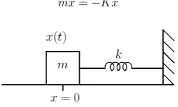
So let us start discussing the simple lumped element model shown in Fig. 1.1. A massless spring of stiffness k is connected on one side to an ideal constraint and to a rigid body of mass m on the other. If x(t) is the position of the body at time t, then the equation of motion is:

mx¨=−Kx (1.1)

Figure 1.1: Lumped element model of a mechanical oscillator.

and the general solution for the free evolution is

x(t) =x0cos(ωmt+φ) where ωm =

p

k/m (1.2)

The two parameters,x0 andφ, depend exclusively on the initial conditionsx(0) and ˙

x(0), since no additional external force is considered. The movement of the mirror is an oscillation around the equilibrium position at x = 0 with amplitude x0 and phase φ. The total energy of the system can be calculated as:

Em = 1 2mx˙

2 + 1

2kx 2

(1.3) it is positive definite and it vanishes forx= 0 and ˙x= 0. The usefulness of this simple model comes from the fact that it is valid for any potential close to a minimum. Its expansion around a stable equilibrium position is equivalent, to the first non-vanishing order, to a quadratic potential. Moreover, it is possible to easily drop the rigid body assumption by means of the Normal Modes Expansion Model [32]. With it, one can forget about the complexity of the dynamics of a three-dimensional body and take into consideration only a limited number of normal modes, if not only one. The mass will be replaced by an effective mass that depends on the mode under consideration and on how the displacement is actually measured. For the fundamental mode, however, the effective mass is usually very close to the physical mass. More details can be found in the appendix (Sec. A).

In order to obtain a more realistic model one needs to include the effect of losses and the action of external forces. There are several dissipation mechanisms: clamping losses [33], that are due to the absorbtion of the oscillator elastic energy

(13)

1.1 Mechanical oscillator

by the environment (constraints, substrate... ); fundamental anharmonic effects such as thermoelastic damping [34], that is, the dissipation of elastic energy into heat. This effect is particularly important in thin structures but is often negligible at cryogenic temperatures; materials-induced losses, that are due to intrinsic defects in the bulk or the surface of the material [35]; at last, viscous damping, that is, energy loss through collisions with the (residual) gas surrounding the oscillator. This mechanism depends strongly on geometry and on the shape of the specific normal mode (see for example Ref. [36]). All these processes add up incoherently so that the total mechanical quality factor is given by 1/Qtot =PQi withiidentifying individual loss mechanisms.

Let us consider the case of viscous damping. The equation of motion for a single normal mode is

¨

x(t) +γmx˙(t) +ω2mx(t) =

Fext(t)

mef f

(1.4) whereγm =ωm/Qmis the (energy) damping rate whileFext(t) represents the sum of all external forces acting on the mechanical oscillator. Even when no deterministic force is present, one needs at least to take into consideration stochastic forces. In particular, a term that is always present is the thermal Langevin force.

Since thermal noise is a fundamental noise source it is necessary to discuss it in more details. Assuming thermal equilibrium between the mechanical oscillator and a reservoir at temperature T, the Langevin force Fth is a stationary Gaussian noise for which the following relations, given by the Fluctuation-Dissipation Theorem (FDT) [37, 38], must hold

hFth(t)i= 0

hFth(t)Fth(t0)i= 2kBT mef fγmδ(t−t0)

(1.5)

-the bracketsh...i denote the average over the statistical distribution of the noise-. To solve Eq. 1.4 it is convenient to work in the frequency space, thus we define the truncated Fourier transform as

xT(ω) = √1

τ

Z τ

0

x(t)eiωtdt. (1.6)

Averaging over independent realizations of xT(ω) one obtains the spectral density

h|xT(ω)|2_i_{. Now, in the limit of}_τ _{→ ∞}_{, under the assumption that}_F

(14)

Using the definition just mentioned, the displacement PSD is given by

Sxx(ω) =

Z ∞

−∞

hx(t)x(0)ieiωtdt. (1.7) At this point, we can use standard input-output theory for linear time-invariant systems to evaluate the mechanical impulse response function whose Fourier trans-form1_{, namely the mechanical susceptibility}2_{, is}

χ(ω) = 1

mef f

1 (ω2

m−ω2)−iωγm

(1.8)

so that Eq. 1.7 becomes

Sxx(ω) =|χ(ω)|2

Z ∞

−∞

hFth(t)Fth(0)ieiωtdt =|χ(ω)|2Sf f,th

(1.9)

whereSf f,th= 2kBT mef fγm is evaluated from Eq.1.5. Looking at Eq.1.9 is already possible to see that in order to have negligible thermal noise (that is low decoherence) is important to have a high mechanical quality factor. Another important result that can be obtained from Eq. 1.9 is that the area under the spectral peak at ωm gives the variance of the displacement noise, that is

1 2π

Z ∞

−∞

Sxx(ω)dω =hx2i. (1.10) In the case of low losses the displacement variance is set by the equipartition theorem, so that hx2i=kBT /mef fωm2

1.1.2

Quantum description

When moving to quantum mechanical formalism [39] the physical quantities position

xand momentumpare replaced by the observables ˆX and ˆP obeying the commuta-tion relacommuta-tion [ ˆX,Pˆ] =i_~. Thanks to the principle of equivalence in the Heisenberg representation, the Hamiltonian operator of the system in Fig. 1.1 is obtained by substituting the corresponding observables in the classical expression of the total energy, so that

ˆ

Hm = ˆ

P2 2m +

1 2k

ˆ

X2 (1.11)

1_{Unless otherwise specified the convention used for the Fourier transform is the following:}

x(ω) =R∞

−∞x(t)e

iωt_dt _and _x₍_t_{) =} 1 2π

R∞

−∞x(ω)e −iωt_dω 2_{Note that for an high}_Q

moscillator the near resonance response can be approximated with a

Lorentzian curve.

(15)

It is convenient to introduce the dimensionless operators ˆxand ˆp, obtained with the normalizations ˆ x= r mωm ~ ˆ

X pˆ=

r

1

~mωm ˆ

P (1.12)

satisfying the relation [ˆx,pˆ] =i. One can also define thecreation ˆb†andannihilation

ˆ_b _{operators as}

ˆ

b = √1

2(ˆx+ipˆ)

ˆ

b†= √1

2(ˆx−ipˆ) (1.13) with commutation relation [ˆb,ˆb†] = 1. Using the latter operators, the Hamiltonian of the system can be rewritten as

ˆ

Hm =~ωm

ˆ_b†_ˆ

b+1 2

. (1.14)

The number operator ˆN = ˆb†ˆb has the same eigenfunctions as the Hamiltonian and it can be show that its eigenvalues are all the natural numbers. The eigenvalues of the Hamiltonian form a discrete ensemble

En =~ωm

n+1 2

with n= 0,1,2, ... (1.15) and corresponding eigenfunctions

ψn(x) = 1

√

2n_n_!

mω_m

π_~

1/4

e−x

2

2 H_n(x) (1.16) where the functions Hn(x) are Hermite polynomials. The first few eigenfunction are shown in Fig. 1.2. If we denote by fn(x) the probability density to find the oscillator between x and x+dx, then fn(x) = |ψn(x)|2_{. It is easy to verify that,} any given state n, the mean position hXˆin =

R

xfn(x)dx and mean momentum

hPˆin = −i~ R fndψn vanish3. On the other hand we can evaluate the root-mean-square value of the position ∆ ˆXnand of the momentum ∆ ˆPnfor a generic eigenstate

n, and find

∆ ˆXn =

q

hXˆ2_i

n− hXˆi2n=xzpf

s

n+ 1 2

∆ ˆPn =

q

hPˆ2_i

n− hPˆi2n =

~

xzpf

s

n+1 2

(1.17)

wherexzpf =

p

~/2mωm is the zero-point motion. From these two equations we can recover, as a consequence of the commutation relation, the Heisenberg inequality

∆ ˆX∆ ˆP ≥ ~

2. (1.18)

(16)

Ifn= 0, then equality holds so that the only minimum uncertainty state among the energy eigenstates is the fundamental one. Up until now we have been discussing a

Figure 1.2: Potential energy and contour of the first few eigenfunctions for an harmonic oscillator.

very ideal case. In order to get a more realistic description we need to include in the model some loss mechanism. The first step is to drop the implicit hypothesis that the oscillator is perfectly isolated. A realistic system is always coupled, in some way, to a high (thermal) energy environment. Formally the Hamiltonian of the system is written as ˆHm+ ˆHenv+ ˆHc where

ˆ

Henv=

X

i

~ωi

ˆ

d†_idˆi+ 1 2

ˆ

Hc=

X

i

~κidˆ †

iˆb+h.c. (1.19) The term ˆHenv describes the environment as an infinite ensemble of harmonic oscil-lators while the term ˆHc describes the coupling between the two subsystems. Note that this means that a state of the harmonic oscillator is not an eigenstate of the global system. Furthermore, there is never enough information on the environment to allow an analytical description of the system and of its dynamics. The only pos-sible approach is a statistical one.

Assuming thermal equilibrium, the global system state is described with a statis-tic ensemble of its different eigenstates, characterized by the density operator

ˆ

ρ= 1

Ze

−_Hˆ_m_/k_B_T

(1.20) where Z is the partition function

Z =T re−Hˆm/kBT

= ∞

X

n=0

e−(n+1/2)~ωm/kBT ₌ e

−_~ωm/2kbT

1−e−~ωm/kbT (1.21)

(17)

from which is possible to calculate the oscillator mean energy at a given tempera-ture T

hHˆmiT =T r

ˆ

Hmρˆ

=_~ωm(nT + 1/2) (1.22) wherenT is the mean number of thermal phonos of the oscillator and is given by

nT = 1

e~kB Tωm −₁

= 1 2coth

~ωm

kBT

− 1

2 (1.23)

a result quite different from the one obtained with classical statistical physics. In-deed, the equipartition theorem attributes to every degree of freedom an energy contribution of 1₂kBT. For an harmonic oscillator the kinetic and potential energy sum up to give a mean energy hHi=kBT. This means that classical and quantum descriptions are equivalent when the temperature is large compared to thequantum temperature TQ, defined as

kBTQ =~ωm (1.24)

while whenT TQ quantum mechanics predicts a minimum energy, the zero point energy, in keen contrast to the vanishing value predicted by classical physics. This can be seen neatly in Fig.1.3. At this point we need to discuss how the coupling to the

Figure 1.3: Mean energy for an harmonic oscillator as a function of bath temperature. Continuous: quantum evaluation. Dashed: Classical calculation.

(18)

in particular concerning the differences with the classical counterpart, but after that, we will assume their validity and directly discuss the results obtained with them.

Eq.1.4is the equation of motion of the system that can be retrieved moving to the Heisenberg picture4_{. But, when writing the correlation function}_R

xx(t) =hxˆ(t)ˆx(0)i is necessary to take into account that the position operator does not commute with itself at different times. Indeed, the correlation function can be expressed as

Rxx(t) =hxˆ(0)ˆx(0)icos(ωmt) +hpˆ(0)ˆx(0)isin(ωmt). (1.25) Classically, the second term in the right hand side (RHS) vanishes since x and p

are uncorrelated for an oscillator in thermal equilibrium. This is not so in quantum mechanics. Using the commutation relation, one can verify that the cross-correlation term is hpˆ(0)ˆx(0)i =−i/2, so that, not only is non-vanishing, but is also complex. The correlation then becomes

Rxx(t) = 1 2

nTeiωmt+ (nT + 1)e−iωmt

(1.26) from which the spectral density can be calculated to be

Sxx(ω) = 2πx2xpf[nTδ(ω+ωm) + (nT + 1)δ(ω−ωm)] (1.27) where we have restored physical units. Note that this expression is not symmetric in frequency. In the classical case the autocorrelation is always a real function from which follows thatSxx(ω) is always symmetric in frequency. As expected, in the high temperature limit nT ' nT + 1 so that classical and quantum predictions coincide. The physical interpretation of this frequency asymmetry can be inferred from the occupation number; the positive frequency part of the spectral density is related to the ability of the oscillator to absorb phonons from the bath, while the negative part is related to the ability to emit phonos5_{. Moreover, when one want to retrieve a}

classical looking equation that relates a stochastic thermal force noise to a damping term in the equation of motion, it is possible to show that it is the symmetric-in-frequency part of the force noise spectrum ¯SF F(ω) = 1₂(SF F(ω) + SF F(−ω)) that causes the oscillator to diffuse while the damping rate is proportional to the asymmetric-in-frequency part of the force noise spectrum, that is γ ∝ SF F(ω)−

SF F(−ω). Note that we introduced thesymmetrized PSD that for an operator ˆA(ω) is defined as

¯

S_Aˆ_Aˆ(ω) = 1

2(SAˆAˆ(ω) +SAˆAˆ(−ω)) (1.28) 4_{For a generic time independent operator ˆ}_A_{the equation of motion is}_A˙ˆ₍_t_{) =}₋i

~[ ˆA, ˆ

H]

5_{An even stronger (heuristic) argument for this interpretation resides in the spectral density of}

the operators ˆb(t) and ˆb†(t), since Sˆbˆb(ω) has a peak centered atω=−ωm while forSˆb†ˆb†(ω) the

peak is centered atω=ωm.

(19)

1.2 The Fabry-P´erot cavity

A deeper insight on the physical meaning of the frequency asymmetry and its inter-pretation can be found again in Ref. [41].

The complete QLEs for a mechanical harmonic oscillator coupled to a thermal bath are given in Eq.1.29. They retain the familiar form of the classical counterpart, associating a stochastic thermal force to a viscous damping force proportional to the velocity. The complete and rigorous treatment can be found in Ref. [42].

˙ˆ

x=ωmpˆ ˙ˆ

p=−ωmxˆ−γmpˆ+ξ

hξˆ(t)i= 0

hξˆ(t) ˆξ(t0)i= γm

ωm

Z _dω

2πe

−iω(t−t0₎

ω

coth

~ω

2kBT

+ 1

(1.29)

Here, γm is the damping rate, as in the classical equation, and ˆξ(t) is a Gaussian quantum stochastic process; its correlation function, expressed in Eq. 1.29, is given by the quantum FDT. In Fig. 1.4 we show the comparison between quantum and classical predictions for the displacement PSD for three temperature values; for

T = 0.1TQthe mean occupation number nT '0 and the displacement PSD is given by the zero point fluctuations. The spectra are normalized to the low frequency value calculated forT =TQ.

Figure 1.4: Comparison between quantum (black) and classical (red) prediction for the displacement PSD normalized toSxx(0) evaluated for T =TQ.

1.2

The Fabry-P´

erot cavity

(20)

latter in Sec.1.2.2. We a interested in the dynamical equations to describe the Fabry-P´erot resonator under the action of both deterministic and stochastic excitations.

1.2.1

Classical description

Consider the simplest cavity composed of two facing partially reflective surfaces with a distanceLbetween them and an electromagnetic monochromatic plane wave of frequency ωl and with direction of propagation normal to both surfaces. The refractive index, both inside and outside the cavity, is n0 = 1. We denote withti(Ti) andri(Ri) the amplitude (power) transmission and reflection coefficients respectively of the i−th surface and with Σ1, Σ2 the fraction of intensity absorbed or diffused by the surfaces. Conservation of energy requires Ri+Ti+ Σi = 1. The transmitted and reflected fields are [43]:

Er =Ein

−r1 +

t2₁r2ei2φ 1−r1r2ei2φ

Et=Ein

t1t2eiφ 1−r1r2ei2φ

(1.30)

whereEin is the amplitude of the field andφ=Lωl/cis the phase difference between the fields at the two surfaces. From these two equations it is possible to define the cavity transmission ˘T and reflection ˘R functions

˘

T = |Et| 2

|Ein|2

= t

2 1t22 (1−r1r2)2

1 1 +Bsin2_φ ˘

R= |Er| 2

|Ein|2

= (ζ/r2)

2₊_B₍₁₋_Σ

1)sin2φ 1 +Bsin2_φ

(1.31)

where we have defined the coefficient B and thecoupling parameter ζ as

B = 4r1r2 (1−r1r2)2

ζ =r2

r1−r2(r21+t21) 1−r1r2

(1.32)

From Eqs.1.31we can see that there are resonant peaks (dips) forφ=nπ, and each peak will have a halfwidth κφ defined by

4r1r2sin2κφ= (1−r1r2)2 (1.33) the distance in frequency between two subsequent peaks is theFree Spectral Range6

F SR=c/2L, so that we can defineκν =κ/2π=κφF SR_2π and the resonance condition can be expressed as ωcav = 2π n F SR. The cavity Finesse is then F = F SR/2κν. The coupling parameter is the fraction of the incident field amplitude that is re-flected at resonance. It distinguishes three regimes: for 0 < ζ ≤ 1 the cavity is

6_{As usual c is the velocity of light in vacuum.}

(21)

said undercoupled, for −1 ≤ ζ < 0 is overcoupled while for ζ = 0 we have optimal coupling.

Particularly important is the case of a cavity with highFinesse. This assumption impliesκν F SR and (Ti,Σi)1 so that we have

F ' 2π

T1+T2+ Σ1+ Σ2 = 2π

T ζ '

T2−T1+ Σ1+ Σ2

T2+T1+ Σ1+ Σ2

. (1.34) The cavity (amplitude) decay rate becomesκ=cT /4Land the transmission and re-flection functions of Eqs.1.31, expressed as a function of the dimensionless detuning ∆n = ∆/κ= (ωl−ωcav)/κ, can be simplified to

˘

T ' 4T1T2

(T1+T2+ Σ1+ Σ2)2 1 1 + ∆2

n

˘

R' ζ

2_{+ ∆}2 n 1 + ∆2

n

. (1.35) We can also define a reflection response function, that in the high Finesse limit is

Hr(∆n) =

Er

Ein

' ζ−i∆n

1−i∆n

. (1.36)

Moreover, the intracavity power at resonance is Pcav(0) =PinF_π(1−ζ) that gives a clear understanding on the regimes definition according to the coupling parameter. In Fig.1.5 we show the cavity response function ˘T and ˘R together with the overall losses 1−R˘−T˘for a given set of parameters (see caption). Up until now we used the

Figure 1.5:Cavity transmission (T˘,blue), reflection (R˘,red) and overall losses (1−R˘−T˘, dashed-green). Values used for the example are T1 = 300ppm, T2 = 25ppm and Σ =

Σ1+ Σ2 = 25ppm.

plane wave approximation for the input field. A real laser beam is similar in many respects, however its intensity distribution is not uniform but is concentrated near the axis of propagation and its phase fronts are slightly curved. Following Ref.[44], each component of the electric field E(x, y, z, t) satisfies the scalar wave equation

(22)

For a field travelling in the z direction one writes E = Γ(x, y, z)e−ik0z _{where Γ is} a slowly varying complex function which represents the difference between a laser beam and a plane wave, that is, a non uniform intensity distribution and its expan-sion with distance of propagation and the curvature of the phase front. Inserting this expression in the wave equation one obtains

∂2

∂x2Γ +

∂2

∂y2Γ−2ik0

∂

∂zΓ = 0 (1.38)

where it has been assumed that Γ varies so slowly with z that the second derivative

∂Γ2/∂z2 can be neglected. We search solutions to Eq. 1.38 of the form Γ =ψ(x, y)·exp

−i

p(z) + k0 2q(z)r

2

(1.39) where, as usual, r2 = x2 +y2. Here, p(z) and q(z) are complex parameters, the first describing the variation of phase along z and the beam divergency, the latter describing the variations in beam intensity with the distancer and the curvature of the phase front.

The solution withψ =constantis the case of a coherent light beam with a Gaus-sian profile and it is perhaps the most important. For convenience one introduces two real parameters R(z) and w(z) related to q(z) by

1

q(z) = 1

R(z)−i

λ

πw(z)2 (1.40)

R(z) is the radius of curvature of the wavefront the intersects the z-axis at z and

w(z) is the decay length of the amplitude with the distance from the axis, called

beam spot: the intensity profile in every beam cross section is a Gaussian curve with width w, whose minimum w0 is called beam waist. In Fig. 1.6(left) is shown the physical interpretation of these parameters. For a free propagating beam, setting the waist in z = 0, we have

w2(z) = w₀2

" 1 + λz πw2 0 2#

R(z) =z

" 1 + πw2 0 λz 2# (1.41)

Higher order solutions of Eq. 1.38 are possible and their space profiles are shown in Fig. 1.6(right). In cartesian coordinate (x, y, z)

ψ(x, y) =Hm(√2x/w)Hn(√2x/w) (1.42) whereHm is the m-th order Hermite polynomial whilemand n are the (transverse) mode numbers. In cylindrical coordinates (r, φ, z)

ψ(r, φ) =√2r/w

l

(23)

Figure 1.6: Left: contours of a Gaussian beam and physical interpretation of the param-eters R(z) and w(z). Right: Different spatial transverse mode. On the center, Laguerre-Gaussian: labels indicate radial and angular nodes. On the right: Hermite-Laguerre-Gaussian: labels indicatex and y nodes.

where Ll_p is a generalized Laguerre polynomial while p and l are the radial and angular mode numbers respectively. In both cases the parameter q evolves along z

as it does for a Gaussian beam, while the phase parameter depends on the order of the specific mode.

An ideal lens leaves the transverse field distribution unchanged but modifies the parameters R(z) and w(z). In order to have a resonance in a cavity the beam must return with the same parameters after a roundtrip. This condition is used to calculate the mode parameters that the beam must satisfy in order to be stable inside the resonator. While q(z) is independent from the mode numbers, p(z) is not, so that different optical modes resonate at slightly different frequencies. The equations derived in the first part of this section are valid for a Gaussian shaped beam (i.e. the fundamental mode T EM00); for higher orders there are increasing deviations [45].

The dynamical equation for the intracavity field is easy to obtain under the assumption of an input field slowly varying on a time scale set by the roundtrip time

τ = 2L/c, so that E(t+τ) = E(t) +τE˙(t) is a valid approximation. Considering a high Finesse cavity and neglecting losses for the moment, after a roundtrip the intracavity field, in a frame rotating atωl, is

E(t+τ) = p1−T1eiωlτE(t) +

p

T1Ein(t+τ). (1.44) Applying the approximation just mentioned, expanding the square root in the RHS and assumingEin(t+τ)'Ein(t) the previous equation became

τE˙(t) = (−κφ+iψ)E(t) +

p

(24)

where we used κφ = T1/2 and ψ is the phase detuning from the cavity resonance, that isωlτ =n2π+ψ. Note that the phase ψ could be due either to a mismatch of the cavity length or a mismatch of the light frequencyψ = 2π∆ν0

F SR+ ∆L λ/2

. Eq.1.45 can be rearranged as

˙

E(t) = (−κ+i∆)E(t) +

r

2κ

τ Ein(t) (1.46)

whereκ is cavity total loss rate. If we drop the assumption of negligible losses, then

κ=κ1+κ2+κΣ7 but the input field is still just coupled through the input mirror. Once solved Eq. 1.46 the reflected and transmitted fields are

E_outr (t) =−Ein(t) +

√

2κ1E(t) Eoutt (t) =

√

2κ2E(t) (1.47)

1.2.2

Quantum description

The quantization of the electromagnetic fields, obtained by expanding the vector potential in terms of cavity modes (see for example [46]), leads to a description based on a simple superposition of independent harmonic oscillators so that quantum states of each mode may be discussed independently. The Hamiltonian of a single cavity mode is

ˆ

H =_~ωcav

ˆ

a†aˆ+1 2

(1.48) with commutation relations appropriate for bosons, that is [â,â] = [â†,aˆ†] = 0 and [â,â†] = 1. Clearly, Eq.1.48 is identical to Eq. 1.14. This means that many aspects discussed in the previous section for the mechanical oscillator will remain valid for the cavity mode. However, before moving to the dynamical equation, let us briefly review some key properties of quantum optical fields.

Some quantum optic basics

In a completely general way, the ensemble of field quadratures can be defined by ˆ

aθ = âe−iθ+ â†eiθ. (1.49) The quadrature operators âθ and âθ+π/2, aside a global phase factor eiθ, allow the identification of the optical phase space with the complex plane with coordinates (hâθi/2,haˆθ+π/2i/2). They are analogous to the position ˆxand momentum ˆp opera-tors and since the commutator for â and â† is non-vanishing there is an Heisenberg

7_Here_κ

i= cT_4Li andκΣ=cΣ_4L with Σ = Σ1+ Σ2

(25)

inequality imposing a lower bound to the product of their uncertainty, namely

∆ˆaθ∆ˆaθ+π/2 ≥1 (1.50)

The eigenstates of the Hamiltonian in Eq. 1.48 are the number or Fock states, in particular, the vacuum state, is defined by ˆa|0i = 0. A more appropriate basis for typical optical fields are thecoherent states. Introduced by Glauber in 1963 [47], these states have an indefinite number of photons which allows them to have a more definite phase than a Fock state where the phase is completely random. Coherent states are generated using the unitary displacement operator ˆD(α), defined as

ˆ

D(α) = exp αˆa†−α∗ˆa (1.51) whereαis a complex number. When ˆD(α) is applied to the vacuum state one obtains

|αi= ˆD(α)|0i. (1.52) If one calculates the expectation values of the quadrature operators for a coherent state one finds hα|âθ|αi = α +α∗ and hα|âθ+π/2|αi = −i(α − α∗) so that α = 1/2hâθ +iâθ+π/2i = Re[α] + i Im[α] which makes evident that the state |αi is merely a translation of the vacuum state to a point α in phase space. It is easy to verify that for a coherent state ∆âθ = 1∀θ.

In order to better understand the connection between coherent states and laser beams, it is useful to introduce the semiclassical description based on the Wigner distribution. This approximation associate to the generic operators Â and Â† two classical pseudo-random variables A and A∗, complex conjugate of one another and having a quasi-probability distribution that coincides with the Wigner dis-tribution [46, 48]. In this way, classical and quantum expectation values coincide when the operators are placed in symmetric order. More precisely, for all symmet-ric functions fS( Â,Aˆ†) of the operators Â and Â† the quantum expectation value

hfS( Â,Aˆ†)i=T r[fS( Â,Aˆ†) ˆρ] is equal to the mean value fS( Â,Aˆ†) defined from the semi-classical variables A and A∗ weighed with the Wigner distributionW(A, A∗) :

fS( ˆA,Aˆ†) =

Z

dAdA∗fS(A, A∗)W(A, A∗) (1.53) The random variableAcompletely characterizes the quantum operator Â, moreover, it can be decomposed into the sum of its mean value A = hAî and a fluctuation termδA=A−A that derives from the quantum nature of Â.

(26)

corresponds to the classical amplitude of the field, and has variance equal to 1 for all quadratures (since ∀θ,∆ˆaθ = 1). A possible realization of the quantum field can be written as

ˇ

α=√Ieiφ (1.54)

so that I = |αˇ|2 _{is the instantaneous number of photons of the field and} _φ ₌

tan−1( ˇαθ+π/2/αˇθ) is the phase of the field. Upon linearization of Eq. 1.54 around the mean value α =

√

Ieiφ is possible to estimate the fluctuations of the quantum intensity δI and phase δφ:

δI =|α|δα_φ δφ= 1

2|α|δαφ+π/2 (1.55)

whereδα_φare fluctuations parallel to the mean field whileδα_φ+π/2 are orthogonal to it. The variance of intensity fluctuations is then ∆I2 ₌_I _{with relative fluctuations} ∆I/I decreasing as 1/

√

I. Since the mean is equal to the variance the statistic is Poissonian, indeed, this is the quantum shot noise and is a direct consequence of the discretization of the field. On the other hand, phase variance is inversely proportional to the mean intensity ∆φ2 _{= 1}_/₄_I_{. Finally, we can recover the} phase-intensity Heisenberg inequality

∆ ˆI∆ ˆφ≥ 1

2 (1.56)

for a coherent state the equality holds since both intensity and phase, independently, have the minimum variance.

A more general class of minimum-uncertainty states are the squeezed states. In general, a squeezed state may have a sub-shot noise variance in one quadrature. The inequality1.56 has to hold so that the variance in the other quadrature has to increase accordingly. They can be generated using the unitary squeeze operator

S(ε) =exp

1 2ε

∗ ˆ

aˆa−1

2εˆa †

ˆ

a†

(1.57)

where=r e2iϕ, so thatrindicates the strength of the squeezing whileϕidentifies its direction in the phase space. The squeezed state|α, εi is obtained by first squeezing the vacuum and then displacing it

|α, εi=D(α)S(ε)|0i. (1.58) The wigner distribution is a bivariate Gaussian distribution, but in this case the variances are different for the two quadratures. Two special cases are worth dis-cussing. When ϕ = φ intensity fluctuations are squeezed while phase fluctuations

(27)

are anti-squeezed; viceversa for ϕ=φ+π/2. If the first case applies, then

∆I =pI e−r ∆φ= e r

2

√

I (1.59)

where it is evident that the inequality1.56holds also in this case. In Fig.1.7is shown a schematic representation of a coherent and a squeezed state. The first experimental observation of squeezed light dates back to 1985 [49].

Figure 1.7: Left: Coherent state. Right: Squeezed state. Here X ≡αθ and P ≡αθ+π/2. The circle and the ellipse are iso-probability curves.

Dynamical equation for a quantum Fabry-P´erot cavity

The equation of motion for the intracavity field in a Fabry-Pérot cavity is obtained by moving to the Heisenberg representation of the Hamiltonian of Eq.1.48, however, as for the mechanical oscillator, for a realistic description of the system dynamics it is necessary to include in the model fluctuation-dissipation processes. Since the Hamiltonian for the optical and mechanical resonators is the same, so could be the treatment in terms of QLEs. The only difference resides in the fact that it is much more convenient to describe the cavity dynamics in terms of the operator â (and â†) since coherent states are its eigenstates.

(28)

ˆ

anew _{= ˆ}_aold_e−iωlt_{) the equation of motion for the intracavity field is}

˙ˆ

a=−(κ−i∆)ˆa+√2κeαin+

√

2κeˆain+

√

2κiˆain,v

hân(t)ân(t0)i=hâ†n(t)â † n(t

0

)i=haˆ†_n(t)ˆan(t0)i= 0

hˆan(t)ˆa†_n(t0)i=δ(t−t0) forn =in and n =in, v

(1.60)

Hereαin=

p

Pin/~ωl is the input field, Pin in the incident power, âin are quantum fluctuations coupled to the cavity mode through the input mirror while âin,v is the vacuum input noise describing all other decay channels (optical losses and transmis-sion through the end mirror). To see how the coupling constant (√κn) between the cavity mode and the ”photon reservoir” is obtained, look, for example Refs. [50,51]. Note that the field operators â and âin have a different normalization, the input field is flux normalized so that hâ†_inâini = Pin/~ωl while the intracavity field in

number normalized so that hˆa†aˆi = nc is number of photons in the cavity at a given time; this means that the intracavity power is given byPcav =~ωlnc/τ. If one compares Eq. 1.60with the classical counterpart in Eq.1.46 the only difference that catches the eye is a factor √τ that accounts for the different normalizations.

Two final remarks have to be made regarding the correlation functions. First, as already stated they preserve the correct commutation relations between opera-tors during the time evolution. Second, they are formally identical to those involv-ing the creation and annihilation operators of the mechanical oscillators, that is,

hâ†(t)â(t0)i = nT δ(t−t0) and hâ(t)â†(t0)i = (nT + 1)δ(t−t0), but at optical fre-quencies nT '0 so that the correlation functions reduce to those listed in Eq. 1.60. Moreover, the cavity mode has more than one decay channel.

1.3

Opto-mechanical coupling

In this section we are going to write the quantum mechanical equations to describe the opto-mechanical interaction. As stated in the previous section we are interested in a one-sided Fabry-P´erot cavity. The mechanical oscillator is also the end mirror of the cavity so that it feels the radiation pressure force F = 2P/c exerted by the intracavity field. Under the action of this force, the cavity length changes from Lto

L+X and in turn the intracavity power is modified since the resonance condition is different. We have already seen the dependence of detuning on length variations. With these two simple considerations it is already possible to write the coupled equations that describe the system in the semiclassical approximation but, since we

(29)

1.3 Opto-mechanical coupling

have already laid the groundwork, we will directly move to the quantum mechanical case.

In the following we will assume that the mechanical oscillator motion is slow compared to the round trip time of a photon in the cavity (adiabatic approximation). In this way it is possible to keep considering only one optical mode. The Hamiltonian operator for the coupled system is

ˆ

H =_~ωcav(X)ˆa†a+~ωm

ˆ_b†_ˆ

b+ 1 2

. (1.61)

The cavity resonance frequency is modulated by the (small) motion of the mirror, in other words the coupling is parametric. Note that the 1/2 term for the optical mode is missing. The reasons are two: first, when moving to the Heisenberg representation its contribution disappears. Note that the same apply to the mechanical mode; second, a more formal derivation (see Ref. [52]) shows that it gives rise to a Casimir term when one accounts for the different density of optical modes inside and outside the cavity. This term, however, can be safely neglected for most opto-mechanical experiments up to date.

Since generally one can safely assume small displacements compared to the cavity length, we can expandωcav(X)

ωcav(X)≈ωcav +X

∂ωcav(X)

∂X +... (1.62)

generally it is enough to keep the linear term. For the simple cavity we are considering

∂ωcav(X)/∂X = −ωcav/L, reflecting the fact that we are defining X > 0 for an increase of the cavity length that in turn leads to a decrease inωcav. The Hamiltonian in Eq.1.61 can be written as

ˆ

H =_~ωcavˆa†a+ 1

2~ωm xˆ

2_{+ ˆ}_p2

−_~g0xˆˆa†a (1.63) where we have defined g0 =

√

2xzpfωcav/L. In the previous equation it is easy to identify the interaction Hamiltonian as

ˆ

Hint =−~g0xˆaˆ†ˆa (1.64) where it is possible to see that the cavity opto-mechanical interaction is funda-mentally a nonlinear process. The radiation pressure force, then, is given by ˆF =

−dHˆint/dXˆ.

(30)

described as a coherent state. We just need to add to the QLEs in Eqs. 1.29 and Eqs. 1.60 the coupling term obtained from Eq. 1.64. In the frame rotating at the laser frequency ωl the coupled equations of motion are

˙ˆ

x=ωmpˆ ˙ˆ

p=−ωmxˆ−γmpˆ+g0ˆa†ˆa+ξ ˙ˆ

a=−[κ−i(∆0+g0xˆ)] ˆa+

√

2κeαin+

√

2κeaˆin+

√

2κiˆain,v

(1.65)

with correlation functions at temperature T

haˆn(t)ân(t0)i=hâ†n(t)â † n(t

0

)i=hˆa†_n(t)ˆan(t0)i= 0

haˆn(t)ˆa†_n(t0)i=δ(t−t0) for n=in and n =in, v

hξˆ(t)i= 0

hξˆ(t) ˆξ(t0)i= γm

ωm

Z

dω

2πe

−iω(t−t0)_ω

coth

~ω

2kBT

+ 1

(1.66)

where ∆0 is the detuning for a vanishing optomechanical coupling. All noise terms considered are unavoidable fundamental noise sources. However in a realistic scenario two additional technical noises can play a relevant role: (i) amplitude noise, which is taken into account assuming αin → αin+αI(t), where αI(t) is a real, zero-mean Gaussian stochastic variable; (ii) phase/frequency noise, which is caused both by the laser frequency fluctuations, and by the fluctuations of the cavity length (and therefore of its resonance frequency) which are not due to the considered mode of the mechanical resonator. The latter are typically much more relevant and can be described writingωl−ωcav →∆0+ ˙φ(t), where ˙φ(t) is a zero-mean frequency noise. As a consequence eqs.1.65 become

˙ˆ

x=ωmpˆ ˙ˆ

p=−ωmx−γmp+g0ˆa†ˆa+ξ ˙ˆ

a=−hκ−i∆0+ ˙φ+g0xˆ

i

ˆ

a+√2κeαin +√2κeαI+

√

2κeˆain+

√

2κiˆain,v

(1.67)

Amplitude noise acts as additive noise on the cavity modes, while frequency noise is a multiplicative noise, affecting the cavity field in the same manner of the fluctuations of the resonator position ˆx.

We want to generate and manipulate optical quantum fluctuations and therefore we consider the motion of the system around a steady state characterized by the intracavity electromagnetic field in an approximate coherent state of amplitude αs, and the micro-oscillator at a new positionxs, by writing:

ˆ

x=xs+x pˆ=ps+p ˆa=αs+a (1.68)

(31)

Substituting Eqs.1.68in Eq.1.67, and retaining only the 0−th order contributions one gets

ps = 0 xs =

g0

ωm

|αs|2 αs=

√

2κe

κ−i∆αin (1.69) where ∆ = ∆0+g20|αs|2/ωm. The exact QLE for the fluctuation operators x,p and

a are given by ˙

x=ωmp ˙

p=−ωmx−γmp+g0(αsa†+α∗sa) +ξ+g0a†a ˙

a=−(κ−i∆)a+i g0αsx+iαsφ˙+i g0x a+iφa˙ +√2κe(αI+ain) +

√

2κiain,v

(1.70)

The nonlinear terms are g0a†a, i g0x a and iφa˙ . The first two terms have negligible effect when |αs| 1, which is usually satisfied, and therefore they can be safely neglected. The last term is a multiplicative noise term and it is not obvious if and when it can be neglected since its evaluation requires the knowledge (or realistic hypotheses) of the frequency and displacement noise spectrum on a wide frequency range. Its treatment is outside the purpose of this thesis and we shall neglect this last term in the following. Keeping only linear terms Eqs. 1.70 become

˙

x=ωmp ˙

p=−ωmx−γmp+g0(αsa†+α∗sa) +ξ ˙

a =−(κ−i∆)a+i g0αsx+

√

2κe˜ain+ Ξ

(1.71)

where we have introduced two noise terms Ξ =iαsφ˙+

√

2κiain,v ˜

ain =ain+αI

(1.72)

describing all detrimental fluctuations acting on the cavity field. At this point we can use Eq.1.47to evaluate the reflected field, that is,aout =−˜ain+

√

2κea. Taking the Fourier transform of Eqs.1.71 and solving for a(ω) and x(ω) one gets

aout(ω) =A1(ω) ˜ain(ω) +A2(ω) ˜a † in(ω)

+A3(ω) Ξ(ω) +A4(ω)Ξ†(ω) +AT(ω)ξ(ω)

x(ω) =B1(ω)

√

2κea˜ † in+ Ξ

†

+B2(ω)

√

2κe˜ain+ Ξ

+χef f(ω)ξ(ω)

(32)

where we have defined the transfer functions

A1(ω) =

−1 + 2κe

K(ω)

1 +i g₀2|αs|2

χef f(ω)

K(ω)

A2(ω) = 2κe

K(ω)

i g₀2α2_sχef f(ω) K∗₍₋_ω₎

A3(ω) =

√

2κe

K(ω)

1 +i g₀2|αs|2

χef f(ω)

K(ω)

A4(ω) =√1

2κe

A2(ω)

AT(ω) =

√

2κe

K(ω)[i g0αsχef f(ω)]

B1(ω) =g0αs

χef f(ω)

K∗₍₋_ω₎

B2(ω) =g0α∗s

χef f(ω)

K(ω)

(1.74)

with K(ω) =κ−i(∆ +ω) and where

χef f(ω) =ωm

ω2_m−ω2−i γmω+i ωmg20|αs|2

1

K∗₍₋_ω₎− 1

K(ω)

−1

(1.75) is the effective mechanical susceptibility modified by the opto-mechanical coupling. At this point we are finally ready to discuss some key aspects of the opto-mechanical interaction.

Bistability

When looking at the steady state solution expressed in Eqs. 1.69 it is possible to verify that trying to calculate the mean number of photons in the optical mode one ends up with a third-degree equation, that is

nc

κ2+ ∆2₀+ 2g 2 0∆0

ωm

nc+

g₀4 ω4 m

n2_c

= 2κe|αin|2. (1.76) This means that above a certain threshold the system shows a bistable behavior. This is due to the radiation pressure force that modifies the potential felt by the mechanical oscillator to the point where it shows two minima. Note that the same effect can be generated by photothermal forces [53].

Dynamical backaction

For a given detuning of the input field from the cavity resonance, the intracavity field exerts a radiation pressure force on the mechanical oscillator. Under the action

(33)

Figure 1.8: Opto-mechanical bistability. The curve represents the mean number of intra-cavity photonsnc as a function of the dimensionless empty cavity detuning ∆0/κ. Dashed line indicates the unstable region.

of this force the mean position of the oscillator is changed, in turn this modifies the optical resonance and thus the intracavity power and the radiation pressure that goes with it. This closed loop effect, usually referred to asdynamical backaction, is completely described in the definition of the effective mechanical susceptibility in Eq. 1.75. The intracavity field essentially modifies the spring constant felt by the mechanical oscillator. Indeed, we can define the optical spring [54,55] as

Kopt =m ωopt2 =m Re

iωmg02|αs|2

1

K∗₍₋_ω₎ − 1

K(ω)

=2mωmg02|αs|2∆

κ2_{+ ∆}2₋_ω2 (κ2_{+ ∆}2₋_ω2₎2_{+ 4}_κ2_ω2

(1.77)

The sign of the optical spring depends on the detuning ∆ of the input field. When ∆< 0 (red-detuned) the mechanical spring is ”softened” so that the effective me-chanical resonance frequency decreases, viceversa, for ∆ > 0 (blue-detuned) the mechanical spring is ”hardened”.

(34)

can define the optical damping rate as

γopt =− 1

ωIm

iωmg20|αs|2

1

K∗₍₋_ω₎− 1

K(ω)

=− 4ωmg

2

0|αs|2κ∆ (κ2_{+ ∆}2₋_ω2₎2_{+ 4}_κ2_ω2

(1.78)

so that the total mechanical damping rate becomes

γom =γm+γopt (1.79) the mechanical effective susceptibility can be written as

χef f(ω) =

ωm (ω2

m+ωopt2 −ω2−iωγom)

. (1.80)

A clean experimental evidence of these two effects in an opto-mechanical cavity was reported in 2006 by Arcizetet al.[56]. In Fig.1.9it is possible to see the dependance on the detuning of γom and of the frequency shift induced by the optical spring, for different values of input power. Note that, whenγom vanishes, the system experiences a parametric instability: any fluctuation grows exponentially up to a saturation value, leading to an oscillation of the mirror at constant amplitude. This effect is also referred to asself-induced oscillations (or”mechanical lasing”). This instability can be detrimental if one needs to work at small detunings. When the opto-mechanical coupling (or the input power) is strong enough, the minimum achievable detuning will be limited by the combined effect of frequency and displacement noise since, under the action of these noise sources, the oscillator can move to the unstable region even if the mean position is well outside it. For a given detuning, the ratio between frequency shift and optical damping rate depends on the ratioωm/κ: in theresolved

sideband regime (κ ωm) the backaction effect manifests strongly on the optical damping rate with negligible frequency shift, and viceversa in thebad cavity regime (κωm).

As for the case of active feedback cooling, the effect of the dynamical back action can be viewed as a change in the thermal bath temperature. We define theeffective temperature, assuming small frequency shifts, as

Tef f 'Tinit

γm

γom

=Tinit 1

1 +C (1.81)

where we have introduced the cooperativity C=γopt/γm, a parameter often used as a figure of merit. Note that this expression derives from classical mechanics and it ceases to be valid for sufficiently low Tef f. A complete quantum mechanical treat-ment can be found in Ref. [57].

(35)

Figure 1.9: Opto-mechanical damping ratio (left) and frequency shift (right) as a function of the dimensionless empty cavity detuning ∆/κ for three values of input power. Shaded area corresponds to the unstable domain.

Noise properties of the output field quadratures

Another way to see the opto-mechanical backaction starts from the consideration that, in a Fabry-P´erot cavity, displacement and frequency or phase noise are com-pletely undistinguishable so that amplitude fluctuations of the cavity fields generate phase fluctuations (through the mirror motion) that in turn affect amplitude fluctu-ations. This means that amplitude and phase fluctuations are correlated. In practice, the same process that gives rise to the optical spring and the cooling/heating of the mechanical resonance can generate squeezing. In other words, the output field can present a sub-shot noise statistic. This effect is usually referred to asponderomotive squeezing [6, 7].

The noise spectrum of the quadrature at phaseθ is defined as

2π S_outθ (ω)δ(ω+ω0) = haθ(ω)aθ(ω0)i (1.82) where aθ is given by Eq. 1.49. Since we are using the correlation functions in the Fourier domain, it is useful to write them here (the non-null ones), even if they are derived from Eq.1.66. For quantum operators we have

hain(ω)a † in(ω

0

)i= 2π δ(ω+ω0)

hain,v(ω)a † in,v(ω

0

)i= 2π δ(ω+ω0)

hξ(ω)ξ(ω0)i= 2π δ(ω+ω0)γm

ωm

ω

coth

~ω

2kBT + 1

.

(1.83)

(36)

in a relatively small frequency band centered around the mechanical resonance so that the white noise assumption is a good approximation. The correlation functions in the Fourier domain for the additional amplitude and frequency noise are

hφ˙(ω) ˙φ(ω0)i= 2π S_φ˙_φ˙δ(ω+ω0)

hαI(ω)αI(ω0)i= 2π SαIαIδ(ω+ω

0

). (1.84)

At this point we have all that we need, we just have to substitute Eq. 1.73 into Eq. 1.49 and calculate haθ(ω)aθ(ω0)i. After some algebraic manipulations one finds

S_outθ (ω) =Sain(ω)

|A1(ω)|2+|A2(−ω)|2+ 2ReA1(ω)A2(−ω)e−2iθ

+Sain,v(ω) 2κi

|A3(ω)|2+|A4(−ω)|2+ 2Re

A3(ω)A4(−ω)e−2iθ

+Sξξ(ω)|AT(ω)|2+|AT(−ω)|2+ 2Re

AT(ω)AT(−ω)e−2iθ

+SαIαI(ω)|η1(ω)e

−iθ ₊_η∗ 1(−ω)e

iθ_|2 +S_φ˙_φ˙(ω)|η2(ω)e−iθ +η2∗(−ω)e

iθ_|2

(1.85) where we have defined η1(ω) = A1(ω) +A2(ω) and η2(ω) = iαsA3(ω)−iα∗sA4(ω). Generally the only measurable quantity is the symmetrized spectral density. Using the definition in Eq. 1.28, we haveSθ_out(ω) = S_outθ (ω) +S_outθ (−ω)/2 from which it is possible to evaluate the angleθmin(ω) that minimizes the quadrature spectrum at every frequency, that is

θmin(ω) = 1

2arctan

"

2Sπ/4_out(ω)−S_out0 (ω)−Sπ/2_out(ω)

S0_out(ω)−Sπ/2_out(ω)

#

(1.86)

and using θ =θmin(ω) in Eq. 1.85 one can calculate the minimum attainable PSD

Smin(ω). With our normalizations the output quadrature is squeezed at the fre-quency ω if Smin(ω) < 1. The first observation of squeezed light generated thanks to the opto-mechanical interaction has been reported by Brooks et al. in 2012 [18] who exploited an experimental setup where the role of the mechanical oscillator was played by a cloud of ultra-cold atoms. The same result has been obtained with a macroscopic mechanical oscillator (a photonic crystal) by Chan et al. in 2013 [19] and, later on, an even stronger squeezing has been reported by Purdy [20] et al..

Displacement spectrum

The total displacement Spectrum can be evaluate from Eqs.1.73, Eqs.1.74 and the definitions of the correlation functions for the various noise sources given previously.

(37)

We are going to separate the total spectrum into three contributions: Sth(ω) due to thermal noise,Sq(ω) due to quantum fluctuations of the intracavity field andScl(ω) due to classical amplitude and frequency noise. These can be calculated to be

Sth(ω) =|χef f(ω)|2Sξ(ω)

Sq(ω) = 2κe|B2(ω)|2Sain(ω) + 2κi|B2(ω)|

2_S

ain,v(ω)

Scl(ω) =|i αsB2(ω)−i α∗sB1(ω)| 2

S_φ˙_φ˙(ω) + 2κe|B1(ω) +B2(ω)|2SαIαI(ω)

with

Sxx(ω) =Sth(ω) +Sq(ω) +Scl(ω)

(1.87)

where, to restor physical unit, one just multipliesSxx(ω) by 2x2zpf. The termSth(ω) of the cooled(heated) mechanical resonance, with the right parameters set, can be extremely close to what one would expect from just the zero point motion. The first experimental evidence of a mechanical oscillator on its ground state in an opto-mechanical cavity has been reported only in 2011 by Chanet al. [21]. The termSq(ω) represents the effect of the radiation pressure shot noise (RPSN) that can excite the mechanical resonance and in principle give a contribution dominant with respect to thermal force noise. The first direct observation of its effects in an optomechanical cavity has been reported in 2013 by Purdyet al. [17].

1.3.1

Noise budget

In this section we want to discuss the different contributions of the various noise sources to the quadrature of the reflected field and the displacement spectrum of the mechanical oscillator. To do this, we are going to use opto-mechanical parameters that are relevant to our experimental setup, as we will show in the next chapters. For the mechanical oscillator these are: effective massm= 10−7Kg, resonance frequency

ωm/2π = 105Hz and a quality factor of Q = 106. As for the optical parameters, we are going to consider an input field of wavelength λ = 1064nm with power

Pin = 1mW, a cavity of length Lcav = 0.5mm with optimal coupling, that is

ζ = 0, and power transmission coefficients Tm = Tl = 50ppm, where Tl includes optical losses due to absorption, diffusion and transmission through the end mirror (oscillator). With these parameters we are consideringF SR= 300GHzand a cavity half-linewidth κ/2π = 2κe/2π = 2κi/2π = 2.4M Hz so that the optical Finesse is

F '63000.

(38)

thermal equilibrium with a bath at the liquid Helium temperatureTbath = 4.2K. As for the classical amplitude noise we consider an input power PSD that is 3dB over the shot noise at P0 = 20mW, meaning that we have SαIαI(ω) =Pin/4P0. The overall

frequency noise is a combination of displacement noise due to other modes of the sys-tem not directly included in the model and the actual excess frequency noise of the input field. We assume for the former Sdisp_˙

φ (ω) = g 2 0(5 10

−35_m2_/Hz_{) (}_rad/s₎2_/Hz while for the latter we use Sαin

˙

φ (ω) = 0.5Hz

2_/Hz_{. The total frequency noise PSD} is then S_φ˙_φ˙(ω) = S_φdisp_˙ (ω) + (2π)2S_φα_˙in(ω). The remaining free parameters are the detuning and the angle θ that defines the quadrature we want to analyze. We fix the former to ∆n = ∆/κ = −0.01, in this way the mechanical resonance is cooled and shifted to lower frequencies. The latter is fixed at θn =θmin(ωm) =−18mrad. Note that all given spectral densities are bilateral.

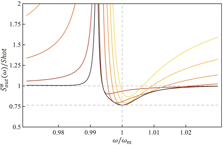
Figure 1.10: The black curve is Smin(ω) while the curves from red to yellow are S θ out at fixed values of θ, increasing from −20mrad(red) to −16mrad (yellow) with steps of 1mrad. All curved are normalized to the shot noise level (dashed gray line). The lower dashed line indicates the maximum squeezing '0.75.

Before discussing the noise budget, we show in Fig. 1.10 the optimum spectrum

Smin(ω) together withS θ

out for different values ofθ around θn. Note that S θ

out is the only measurable quantity (for example with homodyne detection) and by changing

(39)

θ, that is choosing a different quadrature of the output field, one can control the maximum measurable squeezing and its bandwidth.

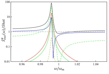
Figure 1.11: Noise budget of Sθ_out (Black) with θ =θn. All noise sources contributions are shown: thermal ξ(red), quantum input ain(green), vacuum fluctuations ain,v (blue), classical amplitudeαI(dashed-dark yellow) and classical frequency noise (dashed-green).

(40)

contribution at thebare mechanical resonance frequency(see Chap.5). Finally, clas-sical amplitude noise (dashed-yellow) gives a negligible contribution for the chosen parameters but particulare care has to be taken to reach the assumed value for

SαIαI(ω).

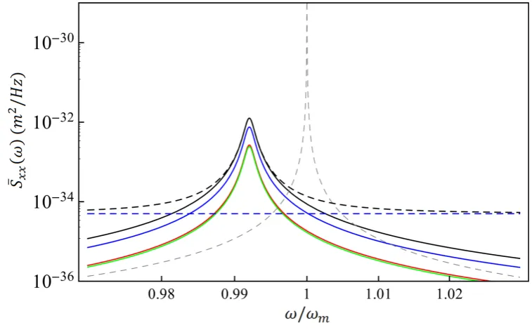
Figure 1.12: Noise budget of Sxx(ω) (Black). All noise sources contributions are shown: thermal (red), quantum (green) and classical (blue). We also show the nominal thermal noise of the free oscillator gray), the frequency/displacement noise floor (dashed-blue) and the ”measurable” total displacement noise (dashed-black).

We show in Fig.1.12the noise budget forSxx(ω) (black). The mechanical spectral peak is shifted to lower frequencies, with ωef f = 99.2kHz, has an effective quality factor Qef f = 750 (cooperativity C = 1.33 103) and an effective temperature of

Tef f = 3.1mK(hnTi = 650). The quantum backaction Sq(ω) (green) and thermal noise Sth(ω) (red) give an equivalent contribution implying that, in principle, the direct effect of RPSN could be measurable. However, the classical excess noiseScl(ω) (blue) is the dominant term and can easily mask the RPSN contribution. As for the quadrature spectra, classical amplitude noise is negligible so that Scl(ω) is entirely due to frequency noise.

Measurements of the displacement PSD are usually performed with interferomet-ric techniques, typically the Pound-Drever-Hall (PDH) detection scheme [58, 59], where the frequency noise (dashed blue line in Fig. 1.12) behaves as an additive

(41)

(42)

(43)

Chapter 2

Design and fabrication of low loss

MOMS resonators

In this chapter we describe the design strategies and the developed fabrication pro-cess of opto-mechanical devices specifically designed to ease the detection of pon-deromotive squeezing. As we have seen in the previous chapter, the main difficulty for the observation of this phenomenon is due to the overwhelming effects of classical noise sources of thermal origin with respect to the weak quantum fluctuations of the radiation-pressure. Therefore, a low thermal noise background is required, together with a weak interaction between the micro-mirror and this background (i.e., high mechanical quality factorsQ). The device should also be capable to manage a rel-atively large amount of dissipated power at cryogenic temperatures (down to a few K).

In the development of our opto-mechanical devices, we are exploring an approach focused on relatively thick silicon oscillators with high reflectivity coating [60, 61]. The relatively high mass is compensated by the capability to manage high power at low temperatures (down to 1 K), owing to a favorable geometric factor (thicker connectors compared to other commonly used devices) and the excellent thermal conductivity of silicon crystals at cryogenic temperatures [62]. Many experiments have demonstrated that silicon mechanical resonators (10×10×10 cm3) can show at such temperatures a loss angle, that models structural damping, as small as

(44)

Chapter 2. Design and fabrication of low loss MOMS resonators

temperature. Indeed, a quality factor of the order of∼106 _{should be high enough to} allow, in principle, the detection of squeezed light in the 100kHz frequency range, as we have shown at the end of Chap. 1.

Actually, for our latest generation of devices, we measured mechanical quality factors up to 2 106 and optical finesse ranging from F ' 4 104 to F ' 6.5 104 at cryogenic temperatures. These results are published in Refs. [24,25, 26].

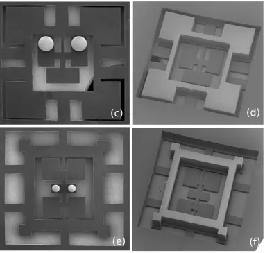
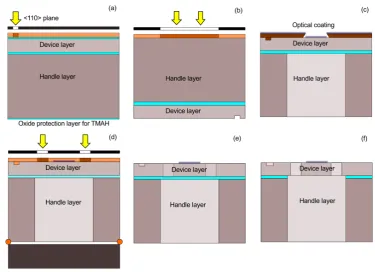
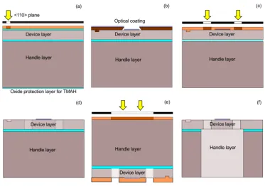
In Sec. 2.1 we present the design strategy used to develop the micro-resonators that allowed us to obtain the results just mentioned. In particular, we devised three novel geometries. In Sec.2.2 we describe the fabrication steps specifically developed to integrate the high-reflective coating deposition(See Ref. [27]).

2.1

Design strategy

According to the description of the cavity dynamics, some fundamental requirements for the oscillator may be derived by comparing the power spectral density (PSD) of the radiation-pressure noise and the PSD of the thermal noise. For instance, in view of the production of ponderomotive squeezing, we require that the radiation-pressure force noise, due to qu