Crowd Motion Analysis: Segmentation, Anomaly Detection, and Behavior Classification

(1)

CROWD MOTION ANALYSIS:

SEGMENTATION, ANOMALY

DETECTION, AND BEHAVIOR

CLASSIFICATION

Habib Ullah

Advisor: Nicola Conci, PhD

(2)

(3)

Abstract

The objective of this doctoral study is to develop efficient techniques for flow segmentation, anomaly detection, and behavior classification in crowd scenes. Considering the complexities of occlusion, we focused our study on gathering the motion information at a higher scale, thus not associating it to single objects, but considering the crowd as a single entity. Firstly, we propose methods for flow segmentation based on correlation features, graph cut, Conditional Random Fields (CRF), enthalpy model, and particle mutual influence model. Secondly, methods based on deviant orientation information, Gaussian Mixture Model (GMM), and MLP neural network combined with GoodFeaturesToTrack are proposed to detect two types of anomalies. The first one detects deviant motion of the pedestrians com-pared to what has been observed beforehand. The second one detects panic situation by adopting the GMM and MLP to learn the behavior of the mo-tion features extracted from a grid of particles and GoodFeaturesToTrack, respectively. Finally, we propose particle-driven and hybrid appraoches to classify the behaviors of crowd in terms of lane, arch/ring, bottleneck, block-ing and fountainhead within a region of interest (ROI). For this purpose, the particle-driven approach extracts and fuses spatio-temporal features to-gether. The spatial features represent the density of neighboring particles in the predefined proximity, whereas the temporal features represent the ren-dering of trajectories traveled by the particles. The hybrid approach exploits a thermal diffusion process combined with an extended variant of the social force model (SFM).

Keywords

(4)

(5)

List of Tables

1.1 Summary of our proposed methods for motion segmentation, anomly detection and behavior classification. Methods deal-ing with any of the three problems are marked Y (Yes) in

the corresponding column. . . 9 2.1 Summary of the video sequences, in terms of average

num-ber of objects, frames per second, numnum-ber of frames, and

resolution, from the UCD dataset. . . 32 2.2 Quantitative comparison of the reference methods and the

proposed method against the ground truth in pedestrian flow segmentation regarding PETS2009, UCSD, and UCD datasets, respectively. The F-scores for individual video se-quences, the average F-score for each datasets, and the av-erage F-scores for all the dataset are provided. The F-scores are shown in bold letters where we outperform the reference

methods. . . 35 2.3 Configuration set for sensitivity analysis for our method. . 39 2.4 Quantitative analysis for our method based on different

para-meter configurations is provided in pedestrian flow segment-ation regarding PETS2009, UCSD, and UCD datasets, re-spectively. The F-scores for individual video sequences, the average F-score for each dataset, and the average F-scores

(10)

2.5 Comparison of our approach with the reference approaches in dominant crowd flows detection. The first column presents the original video sequences and the second column shows the ground truth in terms of four dominant directions and the number of people moving in each dominant direction, re-spectively. Columns {3-6} present the reference approaches

and the proposed approach. . . 49 2.6 Quantitative comparison of the reference approaches and

the proposed approach with the ground truth in terms of accuracies. The first column shows a total number of 31 dominant directions, while other columns present number of correctly detected dominant directions along with percent accuracies by the reference approaches and the proposed

approach. . . 50 3.1 Comparison of our method with the baseline methods. . . 66 3.2 Quantitative analysis for our method based on different

con-figurations is provided in anomaly detection regarding PETS2009, UCSD, and UCD datasets, respectively. The average F-score for each dataset and the average F-F-scores for all the

datasets are provided. . . 68 4.1 Comparison of our method with the reference method in

behavior detection. . . 96 4.2 Comparison of our method with the reference method in

be-havior detection. The average F-scores for each bebe-havior is presented below for the reference method and the proposed

(11)

List of Figures

2.1 CRF Inference . . . 16 2.2 Input frames (first column), CRF segmentation (second column),

and refinement using graph cut (third column). . . 18 2.3 Segmentation. Frames from video sequences (first row);

pure optical flow (second row), correlation [54](third row),

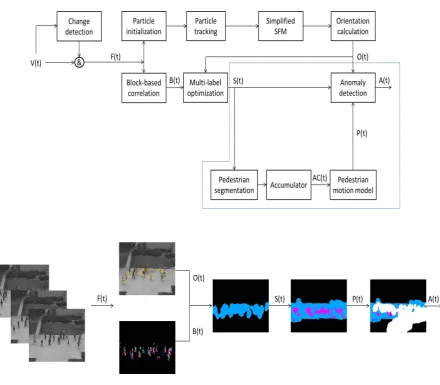
streaklines [32] (fourth row), and our approach (last row) . 21 2.4 Block diagram of the proposed approach representing the

pedestrian flow segmentation and anomaly detection. The output of the major processing stages are indicated using symbolic notations and the output is shown in the lower part of the figure with the help of pictures. For example, V(t),

F(t), B(t), S(t), P(t), AC(t), and A(t) represent the input video, foreground map, block-based correlation, segmenta-tion, pedestrian motion model, accumulator, and anomaly

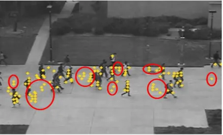
detection, respectively. . . 22 2.5 Noise driven particles, annotated with circles. . . 24 2.6 Application of α-expansion. . . 27 2.7 Movement of the particles from right to left (a) result of the

α-expansion is shown (b) since particles are moving in the

same direction. . . 29 2.8 Segmentation output before (a) and after (b) particle

(12)

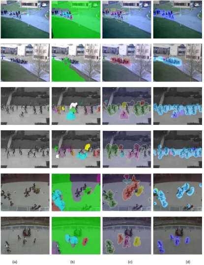
2.9 Pedestrian flow segmentation. A selection of the results are reported in the figure. The first two rows show the per-formance on the PETS2009 dataset, and the central and last two rows report the testing on the UCSD and UCD sequences, respectively. Input frames are shown in column (a), Lagrangian approach [2] in column (b); Streaklines

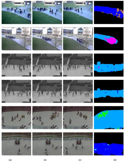
ap-proach [32] in column (c); Our apap-proach in column (d). . 33 2.10 Accumulating motion segmentation. Three frames from two

different sequences in the PETS2009 dataset are shown in the first two rows, UCSD dataset in middle two rows, and UCD dataset in last two rows (columns (a) to (c)); the

ac-cumulated results of our approach are shown in column (d). 34 2.11 Explanation of ground truth calculation. Input frame and

ground truth mask in column (a); Lagrangian results [2] and segmentation mask in column (b); Streaklines results [32] and segmentation mask in column (c); the proposed method

and the corresponding segmentation mask in column (d). 38 2.12 Results of the pedestrian flow segmentation with respect

to different configurations. Each ’o’ symbol presents the average calculated over all video sequences of three datasets. Standard deviations are also plotted representing variations

from the averages. . . 41 2.13 Corner features initialization. Frame from an irregular crowd

video sequence (Left); the same frame with corner features

driven (Right). . . 42 2.14 Interaction flow. The extracted corner features (left column);

the same frame with the interaction flow overlayed (right

(13)

2.15 Orientation-based dominant crowd flows detection. We ana-lyze the crowd flows in eight possible directions according

to the annotations on the left. . . 46 2.16 Example. The top four frames show the motion of a corner

feature to the right side of the image, while the bottom frame

shows the computed tracklet. . . 46 2.17 Orientation information. Input frames from video sequences

(first row); Orientation information annotated with different colors (second row), where each color is associated with a

specific direction. . . 51 2.18 An example of particle initialization (left) and after pruning

(right). . . 52 2.19 Entities grouping. Synthetic example of moving entities (a),

moving entities obtained from the particles mutual influence model (b) and grouping implemented according to the

mo-tion and density features (c). . . 53 2.20 Input frame (a), entities grouping with the zoom on two

sample groups (b). . . 56 2.21 Particle influence and entity grouping. Results obtained on

the UCLA dataset (a) and on the BIWI dataset (b). For visibility, labels are super-imposed on the original frame and

the corresponding grouped entities are zoomed in lower row. 57 3.1 Most representative orientations of motion for two video

se-quences for the assessment of the pedestrian motion model P. Orientations are numbered from 1 to 8, on horizontal axes, representing the angle from 0 to 360 at steps of 45 degrees. Vertical axes represent orientation information accumulated

(14)

3.2 Anomaly detection. Input frames from two video sequences are provided from the datasets: PETS2009 (first two rows), UCSD (middle two rows), and UCD (last two rows) in column (a), whereas detected anomalies are shown in column (b). . 65

3.3 Results of the pedestrian flow segmentation (a) and anomaly detection (b) with respect to different configurations. Each ’o’ symbol presents the average calculated over all video se-quences of three datasets. Standard deviations are also

plot-ted representing variations from the averages. . . 69

3.4 Particles initialization. Frame from video sequence (Left);

frame from video sequence with particles driven (Right). . 70

3.5 Anomaly detection in UMN dataset. Frames taken from four video sequences representing normal behavior of crowd (first row); frames taken from four video sequences representing

abnormal behavior of crowd (second row). . . 74

3.6 Anomaly detection in our UCD dataset. Frames taken from four video sequences representing normal behavior of crowd (first row); frames taken from four video sequences

repres-enting abnormal behavior of crowd (second row). . . 75

3.7 Corner features initialization. Frame from a UCD video sequence where students are walking from left to right (Left column); the same frame from UCD video sequence with

(15)

3.8 Anomaly detection in UMN dataset. Frames taken from four video sequences representing normal behavior of crowd for the reference method and our proposed method (first and second rows, respectively); frames taken from four video se-quences representing abnormal behavior of crowd for the ref-erence method and our proposed method (third and fourth

rows, respectively). . . 79

3.9 Anomaly detection in our UCD dataset. Frames taken from four video sequences representing normal behavior of crowd for the reference method and our proposed method (first and second rows, respectively); frames taken from four video se-quences representing abnormal behavior of crowd for the ref-erence method and our proposed method (third and fourth

rows, respectively). . . 81

4.1 Crowd behaviors. Crowd individuals moving in straight dir-ections representing lanes (first column); individuals mov-ing in curved directions representmov-ing rmov-ings (middle column); individuals from different points accumulating at single

loc-ation representing bottleneck (last column). . . 84

4.2 ROI selection. Drawing a region of interest (a); A grid of particles disposed over the video frame (b); Particle

advec-tion (c); Highlighted paths of particles. . . 87

4.3 Densities of particles at the end of particle advection. Dens-ity of particles in the proximDens-ity remains the same as before representing lane or arch (left); density of particles increased

(16)

4.4 Particle advection. Crowd individuals moving in straight directions representing lane or bottleneck (first column); In-dividuals moving in a noisy straight direction representing lane or bottleneck (middle column); Individuals moving in

curved direction representing ring (last column). . . 89 4.5 Lane. Drawing region of interest manually (first column);

Density of particles converged at the end of particle

advec-tion (second column). . . 91 4.6 Crowd sequences with normal motion. The first and the

third video sequences represent traffic flow and the middle one represents marathon flow. The threshold set to 160

correctly detects the behaviors. . . 92 4.7 Crowd sequences with swift motion. The first video

quence represents the traffic flow and the second video se-quence represents the gathering of people from different dir-ections. The third video sequence represents crowd of people entering a gate. The threshold set to 60 correctly detects the

behaviors. . . 93 4.8 Crowd behaviors. Drawing region of interest manually (first

column); Density map of particles converging at the end of particle advection (middle column); Peak extraction (last

column). . . 94 4.9 Crowd behaviors. Drawing region of interest manually (first

column); Density map of particles converging at the end of particle advection (middle column); Peak extraction (last

column). . . 95 4.10 TDP. The original frame (first column); the motion flow field

(second column) and the coherent motion flow field (third

(17)

4.11 Extended social force model. The original frame from a video sequence (a); the potential particles are annotated in

yellow (b). . . 101 4.12 Crowd behaviors. Lanes are annotated in red (first column),

arches/rings are annotated in green (second column), bot-tlenecks are annotated in brown (third column), blockings are annotated in yellow (fourth column), and fountainheads

(18)

(19)

Chapter 1 Introduction

This chapter overviews the research field investigated in this doctoral study. In particular, we describe crowd motion analysis techniques, focusing on segmentation, anomalies detection, and behavior classification. The main objectives and the novel contributions of this thesis are also presented. Finally, we describe the organization of the thesis.

1.1 Overview

(20)

1.1. OVERVIEW CHAPTER 1. INTRODUCTION

Pedestrian flow implies that the the flow can neither be considered as a continuum, nor can its uniform behavior be verified given that individuals are independent, which are key requirements in the existing techniques. For instance, Ali and Shah [2] proposed a Lagrangian Coherent Structure (LCS) approach to segment the flow using the Finite Time Lyapunov Expo-nent (FTLE) [48], to extract the boundaries between different flow regions in the scene. However, when the optical flow computation is not accurate due to the lack of coherence in motion, the boundaries may be discontinu-ous. Furthermore, the merge operation based on Lyapunov divergence is mainly suitable for combining adjacent segments, resulting also in this case in over-segmented regions in pedestrian flow scenes. A more recent related work [32] proposed streaklines based on linear dynamical model. However, streaklines are incapable to encapsulate the crowd dynamics, thus failing to group pixels with common motion patterns. In addition, streaklines cannot capture temporal changes, exhibiting choppy motion segmentation in high density crowd scenes.

(21)

CHAPTER 1. INTRODUCTION 1.2. PROPOSED SOLUTIONS

the 128-dimensional descriptor [13] [64]. Moreover, the spectral clustering approach fails to simultaneously identify clusters at different scales [35].

Automated detection of anomalous events generated by self-organization phenomena resulting from the unlikely event of a fire or in presence of riots in urban areas, can cause significant hindrance in the flow. This makes necessary to provide more vigilant surveillance, possibly in lieu of, or as an assistance to, human operators. However, there is a lack of empirical studies of crowded scenes where besides basic motion segmentation, also the analysis of more structured behaviors, such as the formation of lanes, or the detection of oscillations at bottlenecks, is decisive for the safety of people during, for example, the access to or exit from mass events, or in situations of emergency evacuation. Congested conditions can possibly trigger crowd disasters arising from the maximum density and irregular flow of crowd. Moreover, the behavior of the crowd may transition from one state of collective behavior to a qualitatively different behavior depending on the density of crowd. Such transitions typically occur when individuals in the crowd accumulate, propagate, or uniformly move with the flow.

1.2 Proposed Solutions

The objective of this doctoral study is to develop efficient techniques for motion segmentation, anomalies detection, and behavior classification con-sidering the complexities of occlusion, foreshortening, and perspective.

Given such requirements, during this doctoral research we contributed in each application scenario proposing the following approaches :

• Motion segmentation;

(22)

1.2. PROPOSED SOLUTIONS CHAPTER 1. INTRODUCTION

extract motion patterns, which are used as a-priori information for CRF training. Training is performed by means of the gradient as-cent algorithm, so as to maximize the conditional likelihood. Further-more, the parameters after training are used for CRF to segment the crowd flow in terms of motion directions. In fact, compared to other approaches, such as Hidden Markov Model (HMM), CRF is able to model dense and correlated flow features of crowd since it models the conditional probability allowing relaxation of the strong independence assumptions made by the HMM.

(23)

represented as a set of nodes of a graph, where each node corresponds to a constituent of a video frame.

Furthermore, we present a novel method [58] for dominant motion analysis in crowded scenes, based on corner features. For this pur-pose, we extract the corner features from a video frame and track them using the Lucas-Kanade optical flow. These features are then analyzed through an enthalpy model returning a subset of features of potential interest. Subsequently, we extract orientation information from the corner features and train a random forest to learn the beha-vior of the crowd, in order to detect dominant motion flows. In fact, random forests deliver a higher level of predictive accuracy automatic-ally, resist to overfitting, diagnose pinpoint multivariate outliers, and exhibit invariance to monotone transformations of variables.

In [46], we detect and track moving entities in wide surveillance videos. Considering the wide area covered by the camera, which makes the detection and tracking of humans, as well as the classification of their motion a complex task and resource consuming, we adopt a particle-based approach to highlight particles of interest and group them particle-based on their motion properties. A cross influence matrix is computed at the particle level identifying the relevant areas of the video, and pruning static particles and outliers. Based on the motion features of the particles marked as interacting with their neighbors, a learning procedure based on an MLP neural network is implemented, in order to create consistent groups, representing the moving entities to be tracked over time.

• Anomaly detection;

(24)

com-1.2. PROPOSED SOLUTIONS CHAPTER 1. INTRODUCTION

pared to what has been observed beforehand. Once the motion flow is extracted from the foreground, an accumulator is constructed on top of each block to create the pedestrian motion model, by collecting evidence regarding the dominant directions of pedestrian motion. The accumulator is updated at every frame, keeping up with the evolution of the pedestrian flow. The pedestrian motion model combined with the output of multi-label optimization and orientation information is exploited to detect anomalies.

(25)

extracted from an arbitrary corner feature is not sufficient to model the abnormal behavior of crowd due to surrounding noise. Therefore, for each corner feature we extract a set of motion features to robustly model the abnormal behavior of the crowd.

• Behavior classification;

We identify crowd behaviors in real-time using a particle-driven ap-proach [56]. We focus on three types of behaviors, namely lanes, arches, and bottlenecks. The method exploits a grid of particles uni-formly distributed on the video frame, and advected over a temporal window through optical flow tracking. Approximating the moving particles to individuals, spatio-temporal features are extracted at the end of the temporal window for each particle within a region of interest (ROI). The temporal features represent the rendering of trajectories traveled by the particles, whereas the spatial features represent the density of neighboring particles in the predefined proximity. The two features are fused together to model the behavior of the crowd in low to medium density crowd. Furthermore, the feature extraction process is computationally affordable, thus suitable to be applied in real-time applications for behavior analysis in crowded scenes.

(26)

in-1.3. THESIS STRUCTURE CHAPTER 1. INTRODUCTION

dividuals on each other, the E-SFM also takes into account the crowd turbulence usually triggered by regions of high interactions. The ap-proach presents significant performance irrespective of the density of the crowd.

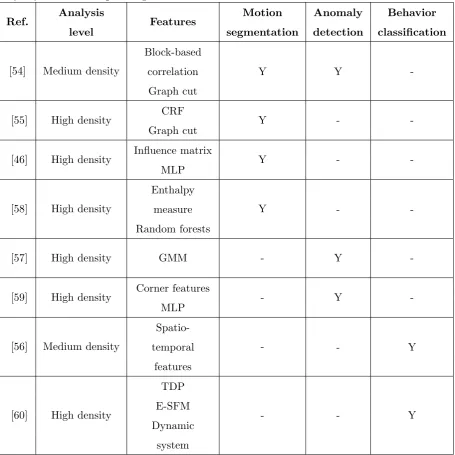
Table 1.1, summarizes our proposed methods covered in this section in terms of analysis and features used for motion segmentation, anomaly detection, and behavior classification.

1.3 Thesis Structure

(27)

CHAPTER 1. INTRODUCTION 1.3. THESIS STRUCTURE

Table 1.1: Summary of our proposed methods for motion segmentation, anomly detection and behavior classification. Methods dealing with any of the three problems are marked Y (Yes) in the corresponding column.

Ref. Analysis Features Motion Anomaly Behavior level segmentation detection classification

[54] Medium density

Block-based

correlation Y Y

-Graph cut

[55] High density CRF Y -

-Graph cut

[46] High density Influence matrix Y -

-MLP

[58] High density

Enthalpy

Y

measure -

-Random forests

[57] High density GMM - Y

-[59] High density Corner features - Y

-MLP

[56] Medium density

Spatio

-temporal - Y

features

[60] High density

TDP

- - Y

E-SFM

Dynamic

(28)

(29)

Chapter 2 Motion Segmentation

This chapter begins with the state of the art regarding motion segmentation and then presents our proposed methods. In particular, the techniques based on block-based correlation, graph cut, and conditional random fields (CRF) are presented. Subsequently, methods for analyzing dominant flows and tracking moving entities based on particle influence model in crowded scenes are presented, respectively.

2.1 State of The Art

(30)

2.1. STATE OF THE ART CHAPTER 2. MOTION SEGMENTATION

descriptors [4] [43] and spatio-temporal volumes [23] [53] [37] [6].

We divide state of the art into three categories based on the density of the flow considered. For example, methods targeting a single individual are under individual level analysis, methods targeting two to five individuals are under low density flow analysis, and methods targeting more than five individuals are grouped under the term high density flow analysis. Meth-ods that rely on individual level analysis and low density flow analysis try to segment individual objects or group of objects in a scene, respectively. These methods tend to produce more accurate results in scenes with a limited number of moving entities. In pedestrian scenes, however, clutter and severe occlusions make the individual or group segmentation an ex-tremely challenging task. In contrast to that, high density flow analysis methods treat the entire scene as a single entity, and usually capable of obtaining coarser-level information, such as the identification of the main flow, disregarding local and finer information.

The methods proposed by Bai and Sapiro [5], Cremers and Soatto [15], and Paragios and Deriche [40], for objects segmentation, fall under indi-vidual level analysis. Bai and Sapiro [5] exploit geodesic transforms to en-courage spatial regularization and contrast-sensitivity for image and video segmentation. The method assumes given user strokes and imposes an im-plicit connectivity prior, which forces each region to be connected to one stroke. In the work by Cremers and Soatto [15], the optical flow constraint is exploited to estimate a conditional probability of the spatio-temporal intensity change. Furthermore, motion estimation and segmentation are integrated into a functional minimization strategy based on a Bayesian framework. A mixture model is exploited by Paragios and Deriche [40] to represent the inter-frame difference. The mixture model comprises of two components corresponding to the foreground and background.

(31)

Vas-CHAPTER 2. MOTION SEGMENTATION 2.1. STATE OF THE ART

concelos [11], and Cisar and Kembhavi [29], segment groups of objects. Cheriyadat and Radke [14] exploited low-level features using optical flow, in order to segment or track the dominant motion in the scene. For this purpose, trajectories are clustered based on a distance measure. Chan and Vasconcelos [11] used a mixture of dynamic textures to fit a video sequence and then assigned homogeneous motion regions to the mixture components. Cisar and Kembhavi [29] perform motion segmentation without relying on the optical flow. For this purpose, they exploit a dynamic texture model to measure the similarity between neighboring spatio-temporal patches. These patches are grouped by connected component analysis, resulting into over segmentation in the presence of pedestrian flow, since patches corresponding to individuals moving homogeneously may not be connec-ted.

(32)

2.2. CRF WITH GRAPH CUT CHAPTER 2. MOTION SEGMENTATION

2.2 CRF With Graph Cut

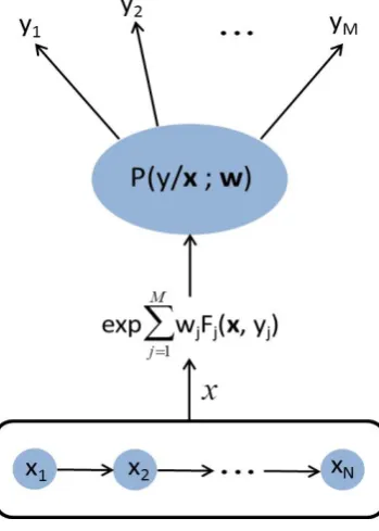
The method we present is modeled in three main stages namely: particle advection, CRF inferencing, and refinement of the motion map using graph cut. During the first stage, a grid of particles is disposed on the video frame. Each particle represents a block of pixels of predefined size. Motion pat-terns, defined in terms of orientation features, are extracted by tracking the particles using the pyramidal Lucas-Kanade optical flow [66]. During this first step, the orientation features act as a sequential data for inferencing the CRF, resulting into a motion map. The orientations features with the corresponding label sequence are used to learn the CRF parameters during the training stage, and the crowd motion directions are inferred on the test samples. In order to provide a more coherent representation of the crowd motion in the second step, graph cut [9] is used to filter out the residual noise.

2.2.1 Inferencing

(33)

CHAPTER 2. MOTION SEGMENTATION 2.2. CRF WITH GRAPH CUT

observation sequence, the CRF thus signals the most probable label in terms of direction, inferring the output label y (y = y1, y2, . . ., yM) of the respective crowd motion direction, and quantized in M possible values.

p(y/x;w) = exp

P

j wjFj(x, y)

Z(x,w) (2.1)

In Eq. (2.1), Fj(x, y) is a feature function, which consists of the paired mapping Fj : X ∗ Y → <. Each feature function renders the score for any output label y in terms of its relevance to the input observation vector

x. The flow of inference process is shown in Fig. 2.1 where N represents the total number of particles tracked. The denominator in Eq. (2.1) is a partition function Z(x,w), which ranges over all the label set y.

Z (x,w) =X y0

exp (

X

j

wjFj(x, y0)

)

(2.2)

Hence, the partition function acts as a normalization factor. Given orientation features x, the corresponding label is obtained as:

ˆ

y = argmaxyp(y/x;w) =argmaxy

X

j

wjFj(x, y) (2.3)

For each j, we will obtain different Fj functions, according to the para-meter wj and the test observation sequence x. Our main contention in obtaining the probability score for each label sequence is that it is easy to reveal the most probable direction for each particle, which can segment the crowd motion as the scene dynamically changes over time.

2.2.2 Training

(34)

Figure 2.1: CRF Inference

to maximize the conditional log-likelihood (CLL) of the set of training examples:

∂ ∂wj

logp(y/x;w) =Fj(x, y)−

∂ ∂wj

logZ(x,w) (2.4) For eachwj, the partial derivative of CLL is evaluated for single training sequences, i.e., one weight for each feature functionFj. The partial derivat-ive with respect to wj corresponds to the i-th value of the feature function for its true label y, minus the averaged values of the feature function for all possible labels y. Therefore, Eq. (2.4) can be rewritten as:

∂ ∂wj

logp(y/x;w) = Fj(x, y)−

X

y0

p(y0/x;w) [Fj(x, y0)] (2.5)

(35)

rate.

wj = wj +α(Fj(x, y)−

X

y0

p(y0/x;w) [Fj(x, y0)]) (2.6)

2.2.3 Sanitizing the motion map

Although the output of the CRF inference is in general quite accurate in indicating the motion flow, it still includes a non negligible amount of noise. In order to remove this noise and to better present the main motion directions of the crowd flow, we exploited the α-expansion moves based on graph cuts [9], which produce a solution within a known factor of the global minimum of the energy function. The minimization process takes place according to Eq. (2.7)

E(L) = X pP

Dp(Lp) +

X

(p,q)N

Vp,q(Lp, Lq) (2.7)

where Dp is the so-called data cost term, and Vp,q is the smooth cost term. The α-expansion minimizes the energy function for a set of labels under the class of smoothness term, called metric. We exploited both the data cost term and the smooth cost terms so that the resulting labeling fit to the data and accomplishes the desired smoothing. Fig. 2.2 presents the effectiveness of the α-expansion moves. Further detail of this process is provided in Section 2.3.2.

As shown in Fig. 2.2, the α-expansion moves demonstrate a very good capability in suppressing the residual noise left by the preceding processing stages.

2.2.4 Experimental results

(36)

eval-2.2. CRF WITH GRAPH CUT CHAPTER 2. MOTION SEGMENTATION

(37)

uate the effectiveness of our proposed approach. In Fig. 2.3, the first rows present the snapshots of the original video sequences, while the second, third, fourth and fifth rows show the results obtained using (i) pure optical flow, (ii) the method in [54], (iii) streaklines approach [32], and (iv) the proposed approach, respectively.

To neglect regions without motion, we discard small magnitude optical flow. For the extraction of the orientation features for each particle, the resolution of the grid is kept half of the resolution of the video frame. For each particle, the orientation features consist of a vector of N = 4 obser-vations, where each element of the vector corresponds to the orientation information extracted after each K = 8 frames. The possible output direc-tions are M = 8, one label every 45◦. When applying the graph cut, each frame processed by the CRF is divided into blocks 2×2 pixels. Each block is considered as a single element and scanning is carried out from top-left to bottom-right. For each central block, the spatial neighborhood is set to 5×5 blocks. For the training phase, we used 800 samples. Each training sample is selected randomly, so that the trained model reflects a relevant and accurate representation of the training data.

We track the particles for 8 consecutive frames by using the Lucas-Kanade optical flow. Then, the obtained tracklets are drawn according to the selected eight possible output directions. It is evident from the seg-mentation map, that the simple optical flow representation is not powerful enough to segment the crowd motion. Also, when comparing with the method presented in [54], we can notice inconsistencies in the crowd mo-tion in Fig. 2.3, and this is evident especially in the first and third video sequences in the first row, where the crowd is moving in semi-circle direc-tion.

(38)

Figure 2.3: Segmentation. Frames from video sequences (first row); pure optical flow (second row), correlation [54](third row), streaklines [32] (fourth row), and our approach (last row)

(39)

CHAPTER 2. MOTION SEGMENTATION 2.3. BLOCK-BASED CORRELATION

quite unreliable results for all video sequences comparing to our approach. We are able to outperform the three methods thanks to the CRF inference, mainly aimed at learning the temporal evolution of the crowd motion, and the graph cut, which consolidates the output in the spatial dimension.

2.3 Block-Based Correlation

We characterize pedestrian flow segmentation from the computer vision point of view by considering the pedestrian flow beyond just a collection of spatially proximate individuals, but also as a dynamic unit that exhibits various properties. In our approach, we have selected different directions of motion where each direction is represented by a label. We represent the input video, foreground frame, orientation information, motion segmenta-tion, and anomaly detection with the symbols V(t), F(t), O(t), S(t), and A(t), respectively. The motion segmentation is obtained by operating on the union of the correlation information with the orientation information, as formulated in Eq. 2.8.

S(t) =B(t)∪O(t) (2.8) An overview of the whole processing chain is shown in Fig. 2.4. The proposed method operates on the foreground region. Therefore, foreground is first extracted from each input frame of the video sequence through the Gaussian mixture model [51]. This is represented as change detection in the first box on the left side of Fig. 2.4. We then correlate the information of the pedestrian flow by applying a block-based correlation technique in the spatio-temporal domain, returning the preliminary segmentation map

(40)

2.3. BLOCK-BASED CORRELATION CHAPTER 2. MOTION SEGMENTATION

(41)

orientations that characterize the pedestrian motion. However, since the multi-label optimization might still contain a residual noise, we integrate the orientation information of the particles, in order to consolidate the output and provide a more consistent representation of pedestrian motion

S(t) as shown in Fig. 2.4. To this aim, we initialize a grid of particles on the foreground region. Each particle represents the position of a pixel, and is tracked using the pyramidal Lucas-Kanade optical flow [66]. In order to identify only the particles that exhibit a relevant motion, we exploit a sim-plified variant of the Social Force Model (SFM) [33]. The SFM describes the motion of particles as if they are subject to social forces. Therefore, the model is able to discard the noise-driven particles, as shown in Fig. 2.5. Each block may be overlapped with an arbitrary number of particles since these particles are not directly associated with blocks. The direction information of the particles is then integrated with the multi-label optim-ization technique in order to provide a more consistent representation of the pedestrian motion, as detailed in the next sections. In fact, a pedes-trian flow can be represented as a set of nodes of a graph, where each node corresponds to a region (block) of the video frame. Considering that the characterization of nodes is relatively simple, we transform the problem of pedestrian flow segmentation into a problem of graph-based optimization. In next sections, we provide the details regarding the steps of the pro-posed algorithm for motion segmentation, namely block-based correlation, multi-label optimization, and simplified social force model.

2.3.1 Block-based correlation

(42)

Figure 2.5: Noise driven particles, annotated with circles.

describes the most likely displacement across two successive time instants. Instead of a pixel-based approach, our choice for the block-based approach is motivated by the fact that it is robust to illumination variations and dynamic background [44].

In order to efficiently exploit the correlation information, an accumu-lator is implemented to store the evolution of each block over time. The comparison of the reference block with each neighboring block in the pre-vious frame is computed on a pixel basis, and formulated according to Eq. (2.9):

Cblock =

X

i,j

1

1 +|pt(i, j)−pt−1(i, j)|

(2.9)

where pt(i, j) and pt−1(i, j) represent the gray scale value of the pixel in

(43)

respectively. For each block, the dominant direction is stored in terms of absolute angle as formulated in Eq. (2.10):

Ψb(θ) = B

X

blocks=b

D

X

directions=i

[θ ==i], (2.10)

W here ∀b ∈ {1, . . . , B},

∀i ∈ {1, . . . , D}

where B and D represent the number of blocks in a frame and possible directions, respectively. The correlation information about the motion dir-ection will be used as input for the pedestrian flow segmentation based on graph-cut, as will be described in Section 2.3.2.

Our choice of implementing block-based correlation to extract a prelim-inary motion map, is preferred to particle advection through optical flow (as in [2] [32]), since the latter might not be appropriate for pedestrian scenes where the background is by definition dynamic, and in which clutter and complicated occlusions often occur. Moreover, optical flow techniques do not provide accurate measures of motion. On the contrary, when observed at block level, pixel intensities in blocks show strong correlation across consecutive frames, thus giving the opportunity to better highlight motion patterns in the pedestrian flow.

2.3.2 Multi-label optimization

(44)

min cut/max flow algorithm proposed by Boykov et al. in [8]. In par-ticular, due to the segmentation problem based on orientations, we used the α-expansion moves based on graph cuts [9]. The α-expansion moves are formulated in terms of energy minimization process according to Eq. (2.11), where Dp is the so-called data cost term, and Vp,q is the smooth cost term.

E(L) = X pM

Dp(Lp) +

X

(p,q)N

Vp,q(Lp, Lq), (2.11)

In this process, the objective is finding the label that minimizes the energy in Eq. (2.11). The data cost represents the appropriateness of a label for the pixel p given the observed data, whereas the smooth cost represents the extent to which labeling is not piecewise smooth. In Eq. (2.11), M and N are the sets of interacting pairs of pixels denoted by p

and q, L represents the label, and Lp and Lq are the labels associated to pixel p and pixel q, respectively.

We show the performance of the α-expansion moves with the help of an example. Considering a sample situation with eight labels (from 0 to 7) as input, the output of the algorithm is shown in Fig. 2.6. As can be seen, 0 and 6 are absorbed by 7 because of the short distance in terms of minimization of the energy function.

Input Output

7 7 7 7 7 7 7 7 7 7

7 0 0 0 7 7 7 7 7 7

3 3 0 6 6 2 2 7 7 7

2 2 1 1 1 2 2 1 1 1

5 5 5 5 5 5 5 5 5 5

(45)

In our implementation, we exploited both the data cost term and the smooth cost term so that the resulting labeling fits the data and accom-plishes the desired smoothing. Each block is labeled in the frame according to the angle information, meaning that each label represents a different mo-tion direcmo-tion. Without loss of generality, and similarly to other approaches proposed in literature, we have selected W = 8 different directions quant-ized with a step of 45 degrees. However, any arbitrary number of elements can be chosen. The data cost assigns different weights to each motion direction extracted by block correlation according to the distance between them. The higher the distance, the higher the data cost. The angle is then compared with the 8 angles of our label set, searching in a neighborhood window of 5x5 blocks.

Given W labels we calculate the minimum distance R between labels as in Eq. (2.12).

R = 360

W (2.12)

The data cost is then computed for each node according to Eq. (2.13).

D(θl) = min θl R − θ R

, N −

θl R − θ R . (2.13)

In Eq. (2.13), θl is the angle (motion direction) in our label set, and θ is the current angle computed as discussed in Section 2.3.1. The angle θ is then compared with all the angles in the label set and the one minimizing the energy function (Eq. (2.11)) is chosen. Furthermore, the smooth cost term is calculated according to Eq. (2.14).

V (θl, θl−1) =|(θl −θl−1)| (2.14)

(46)

energy minimization of graph cut is an effective way to fuse similar motion regions, thus limiting the effect of over-segmentation in pedestrian flows. Compared to the state of the art works presented by Ali and Shah [2] and Mehran et al. [32], this representation introduces some important benefits. For example, FTLE [2] identifies LCS as ridges in the pedestrian scenes. These ridges correspond to the boundaries segmenting the flow. All the particles within each region are considered as showing the same behavior. Following a similar paradigm, streaklines [32] are defined as the loci of particles that have earlier passed through a prescribed point. Streaklines are clustered on the basis of their similarity, to identify segments of the video with similar motion. However, both the boundaries of LCS [2] and streaklines [32] are delineated to combine adjacent segments of the dense scene, often resulting in over segmentation of pedestrian flows.

2.3.3 Simplified social force model

(47)

noise-CHAPTER 2. MOTION SEGMENTATION 2.3. BLOCK-BASED CORRELATION

(a) (b)

Figure 2.7: Movement of the particles from right to left (a) result of the α-expansion is shown (b) since particles are moving in the same direction.

driven particles, because they do not satisfy these requirements. Therefore, a set of potential particles are extracted by exploiting a simplified variant of the Social Force Model (SFM) [33], which measures the internal motiv-ations of the individual particle to perform certain movements, and take into account the influence of the other particle surrounding it.

According to the SFM, the velocity of each particle k with mass mk obeys to Eq. (2.15).

mk

dvk

dt = SFk = SFp,k +SFint,k (2.15)

where SFk is a combination of the personal desire force SFp,k and the interaction force term SFint,k. Considering that each particle in the SFM is treated as an individual in the pedestrian flow, it is assumed that each particle pursues certain goals. Therefore, the personal force of a particle is formulated according to Eq. (2.16).

SFp,k = 1

λ|v

p

(48)

where λ is the relaxation parameter, v_kp is the desired velocity, and vk is the actual velocity of the particle. The desired velocity v_kp is calculated using the Euclidean distance where the initial position and final position of the particle k are considered. The actual velocity vk represents the average velocity calculated over T observations in a fixed temporal window.

The interaction force SFint,k consists of the repulsive force SFrep (to en-sure a certain distance between particles) and an environment force SFenv, to avoid obstacles. In our case, however, we seek to extract potential particles associated to pedestrian motion instead of detecting panic beha-viors of the dense crowd [33]. Therefore, we formulate the interaction force

SFint,k of a particle k according to Eq. (2.17).

SFint,k = hvki (2.17) where hvki is the average velocity calculated over a fixed spatio-temporal window. The size of the spatial window for the neighboring particles is currently set to 3×3. Further details of the SFM are not in the interest of this paper and can be found in relevant citations in [19] [20] [33] for a more comprehensive discussion. To this end, the simplified social force model can be summarized as in Eq. (2.18):

mk

dvk

dt = SFk =

1

λ|v

p

k −vk|+hvki. (2.18) In our model we set both the relaxation parameter λ and mass mk of a particle k to 1 since all particles can be assumed of the same size.

(49)

(a) (b)

Figure 2.8: Segmentation output before (a) and after (b) particle advection representing significant improvement in the performance.

considerable improvement to the pedestrian flow segmentation, as can be seen in Fig. 2.8.

(50)

Table 2.1: Summary of the video sequences, in terms of average number of objects, frames per second, number of frames, and resolution, from the UCD dataset.

Video sequences Avg. objects FPS No. of frames Resolution

S10 15.93 29 1422

320x240

S11 9.37 29 870

S12 5.02 29 1067

S13 5.17 29 933

for both flow segmentation and anomaly detection, as compared to other benchmark datasets lasting only a few seconds. The details of the video sequences are reported in Table 2.1. To evaluate the motion segmentation performance of our approach, we compared it with the state of the art recently proposed by Ali and Shah [2] and Mehran et al. [32].

(51)

(52)

(53)

Table 2.2: Quantitative comparison of the reference methods and the proposed method against the ground truth in pedestrian flow segmentation regarding PETS2009, UCSD, and UCD datasets, respectively. The F-scores for individual video sequences, the average F-score for each datasets, and the average F-scores for all the dataset are provided. The F-scores are shown in bold letters where we outperform the reference methods.

Dataset Seq. No. Lagrangian [2] Streaklines [32] Our method

PETS2009

S1 0.21 0.38 0.54

S2 0.20 0.44 0.52

S3 0.55 0.48 0.58

S4 0.12 0.52 0.53

Average 0.27 0.45 0.54

UCSD

S5 0.30 0.41 0.47

S6 0.27 0.31 0.39

S7 0.30 0.37 0.42

S8 0.23 0.34 0.44

S9 0.43 0.40 0.41

Average 0.30 0.36 0.42

UCD

S10 0.20 0.31 0.48

S11 0.29 0.30 0.42

S12 0.31 0.28 0.27

S13 0.23 0.28 0.42

Average 0.25 0.29 0.39

(54)

rows show the results of two video sequences taken from the UCSD data-set [30], where people are mainly moving from left to right. Furthermore, the last two rows show the results obtained for two video sequences taken from our UCD dataset. The scene refers to a continuous flow of people moving from bottom left to right and right to left, respectively.

As can be seen in Fig. 2.9, both the Lagrangian approach [2] and the streaklines [32] exhibit irregular motion segmentation, especially for the first two video sequences, whereas our approach is spatially and temporally consistent, as well as more accurate. The Lagrangian method [2] tends to segment the motion also when the boundaries in the optical flow field are not salient. The streaklines approach [32], instead, is mainly based on spatial correlation with a frailly temporal component, which turns out to be a discriminant factor. Moreover, streaklines [32] create stilted time lag and cannot detect local spatial changes, hence leaving spatial crevices in flow and abrupt transitions between frames (column (c) in the last two rows of Fig. 2.9). Furthermore, the Lagrangian method [2] can not cope with video sequences where the pedestrian motion is occurring concurrently in different directions. This can be seen in the third and fourth rows, column (b), of Fig. 2.9. Our approach in the column (d) shows that the obtained results are visually consistent with the pedestrian flow. Fig. 2.10 reports the accumulated results obtained using the proposed approach.

(55)

Figure 2.11: Explanation of ground truth calculation. Input frame and ground truth mask in column (a); Lagrangian results [2] and segmentation mask in column (b); Streak-lines results [32] and segmentation mask in column (c); the proposed method and the corresponding segmentation mask in column (d).

.

for flow segmentation are presented in Table 2.2 for each dataset, where the performance evaluation is carried out by comparing our results against the collected ground truth. It is worth noting that most of the datasets do not come with an associated ground truth, as far as the flow segment-ation is concerned, and mostly qualitative evalusegment-ation is used to validate the approaches. However, in order to further demonstrate the validity of our approach, we have collected the ground truth by manually annotating individuals in each video in the pedestrian scene using the RATSNAKE annotation tool [21]. For instance, the ground truth for a video frame, from the PETS2009 dataset, is annotated in the column (a) of Fig. 2.11. The same annotation tool is used to generate the binary masks for the reference methods and the proposed method (column (b) to (d)).

(56)

perform-2.3. BLOCK-BASED CORRELATION CHAPTER 2. MOTION SEGMENTATION

ance is mainly due to the fact that the Lagrangian approach [2] is more oriented towards coherence in pedestrian flow; as the density of the pedes-trian changes over time in a video sequence, the coherence changes as well, making the results less reliable. Similarly, our approach also outperforms the streaklines [32] (fourth column). Significant achievement in the average performance of the the proposed approach can be seen in the last row of Table 2.2.

Sensitivity Analysis

Our method is associated with a few parameters. Therefore we have used different parameter configurations, listed in Table 2.3, for all the tests, in order to demonstrate the robustness of our approach. These configurations are encoded in the experiments based on three sets of block sizes: 2x2, 4x4, and 8x8. For block size equal to 2x2, we have used different temporal win-dows and thresholds ranging from 5 to 15 and from 10 to 20, respectively. In order to investigate the performance of our approach by changing block sizes to 4x4 and 8x8, different thresholds are combined with the temporal window equal to 10. In Tables 2.4, results of our method based on fifteen configurations (C1 to C15) are shown, along with average results for each dataset and the average results for all datasets.

(57)

CHAPTER 2. MOTION SEGMENTATION 2.4. ENTHALPY MODEL

Table 2.3: Configuration set for sensitivity analysis for our method.

Parameters C1 C2 C3 C4 C5 C6 C7 C8 C9 C10 C11 C12 C13 C14 C15

Threshold 10 15 20 10 15 20 10 15 20 10 15 20 10 15 20

Temporal window 5 10 15 10

Block size 2x2 4x4 8x8

with standard deviation for each configuration in column (a) of Fig. 2.12. The plot represents consistent variations from the averages for most of the configurations.

2.4 Enthalpy Model

(58)

2.4. ENTHALPY MODEL CHAPTER 2. MOTION SEGMENTATION

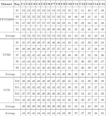
Table 2.4: Quantitative analysis for our method based on different parameter configura-tions is provided in pedestrian flow segmentation regarding PETS2009, UCSD, and UCD datasets, respectively. The F-scores for individual video sequences, the average F-score for each dataset, and the average F-scores for all the datasets are provided.

Dataset Seq. C1 C2 C3 C4 C5 C6 C7 C8 C9 C10 C11 C12 C13 C14 C15

PETS2009

S1 .54 .54 .54 .45 .54 .54 .54 .54 .54 .52 .51 .51 .48 .47 .48

S2 .53 .52 .53 .52 .52 .52 .51 .50 .51 .48 .48 .48 .41 .41 .42

S3 .57 .58 .57 .57 .57 .57 .58 .58 .58 .31 .29 .29 .34 .35 .38

S4 .52 .53 .51 .51 .51 .49 .50 .50 .49 .45 .45 .42 .46 .49 .49

Average .54 .54 .53 .51 .53 .53 .53 .53 .53 .44 .43 .42 .42 .43 .44

UCSD

S5 .45 .47 .48 .49 .47 .48 .46 .46 .44 .43 .43 .43 .29 .29 .34

S6 .38 .39 .38 .38 .38 .37 .37 .37 .37 .31 .31 .32 .27 .28 .29

S7 .42 .42 .42 .42 .44 .42 .41 .41 .40 .40 .38 .37 .32 .34 .36

S8 .43 .44 .43 .42 .39 .39 .42 .42 .42 .35 .35 .36 .29 .29 .27

S9 .41 .41 .41 .41 .38 .42 .38 .39 .41 .33 .33 .36 .39 .37 .37

Average .41 .42 .42 .42 .41 .41 .40 .41 .40 .36 .36 .36 .31 .31 .32

UCD

S10 .48 .48 .48 .48 .48 .48 .48 .47 .48 .45 .45 .45 .38 .39 .38

S11 .42 .42 .42 .42 .42 .42 .42 .42 .41 .36 .35 .33 .25 .27 .31

S12 .27 .27 .26 .26 .26 .26 .26 .26 .25 .20 .20 .19 .23 .23 .29

S13 .42 .42 .42 .42 .42 .42 .42 .42 .41 .40 .40 .39 .27 .27 .28

Average .39 .39 .39 .39 .39 .39 .39 .39 .38 .35 .35 .34 .28 .29 .31

Average .44 .45 .45 .44 .44 .44 .44 .44 .43 .38 .37 .37 .33 .34 .35

(59)

(a)

Figure 2.12: Results of the pedestrian flow segmentation with respect to different config-urations. Each ’o’ symbol presents the average calculated over all video sequences of three datasets. Standard deviations are also plotted representing variations from the averages.

and the corresponding label sequence are used to learn the random forest parameters during the training stage, and the dominant flows are inferred on the test samples.

2.4.1 Corner features extraction

We selected corners as the main feature to analyze, since they represent peculiar elements in the scene and can be easily tracked in dense crowded scenes, leading to better consistency and accuracy in tracking, especially in scenes representing complex motion. The corner features are extracted from the video frame as shown in Fig. 2.13. To detect them, the function formulated in Eq. (2.19) is maximized.

E(u, v) ≈ X

xy

(60)

Figure 2.13: Corner features initialization. Frame from an irregular crowd video sequence (Left); the same frame with corner features driven (Right).

.

intensity at (x, y), and I(x+u, y+v) is the intensity at the moved window (x+ u, y + v). The function in Eq. (2.19) can be reformulated as in Eq. (2.20).

E(u, v) ≈ h u v i

M "

u

v #

(2.20)

Where u is the displacement of the window w along x, and v is the dis-placement of the window w along y. The score R for a corner feature can be determined from the eigenvalues of the matrix M as formulated in Eq. (2.21).

R = λ1λ2 −k(λ1 +λ2) (2.21)

In the equation, k is a free parameter. A window with the greatest R

(61)

2.4.2 Enthalpy model

The objective of this processing stage is to isolate and filter out the corner features that do not contribute to the identification of the dominant crowd flow detection. Motion information, defined in terms of velocity mag-nitudes, is extracted at regular intervals ofK frames by tracking the corner features using the Lucas-Kanade optical flow [66].

The motion patterns observed in a crowded scene can be well modeled through a common thermodynamic measure, the enthalpy. Compared to the entropy model, which measures the disorder of a process, the enthalpy is a measure of the total energy of a thermodynamic system.

In thermodynamics, the enthalpy of a system with respect to temper-ature T and pressure P is formulated in Eq. (2.22).

dH = ∂H ∂T P dT + ∂H ∂P T dp (2.22)

In a thermodynamic system, energy is measured with respect to some reference energy. Therefore, the internal energy U is calculated as a vari-ation in U, instead of an absolute value as formulated in Eq. (2.23).

dU = ∂U ∂T V dT + ∂U ∂V T dV (2.23)

(62)

distinct characteristics represented by the enthalpy model as formulated in Eq. (2.24).

H = U +pV (2.24)

Here, U is the internal energy, p is the pressure, and V is the volume of the system. We exploit the kinetic energy in terms of internal energy, since we are only interested in motile corner features. Pressure is defined as p = F orce/Area and F orce is F = mass ∗ acceleration. For accel-eration, we calculate the average velocity hvi in the spatial neighborhood over time, whereas the area A is the total number of corner features in the spatial neighborhood. Mass and volume of each corner feature may be associated with its contribution in the corresponding subpopulation, in the spatial neighborhood. However, we set them to 1 in our case to maintain consistency. Our enthalpy model is thus formulated in Eq. (2.25).

H = 1

2mv

2

+

∂hvi

∂t

1

A

(2.25)

Figure 2.14: Interaction flow. The extracted corner features (left column); the same frame with the interaction flow overlayed (right column).

.

(63)

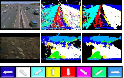
depicted in Fig. 2.14, the orientation information of each corner feature in terms of angle of motion is extracted at regular intervals of K frames. We have selected 8 different directions quantized with a step of 45 degrees as depicted in Fig. 2.15, where R, TR, T, TL, L, BL, B, and BR stand for right, top right, top, top left, left, bottom left, bottom, and bottom right, respectively. The collected orientation features are stored to construct a feature vector for each corner feature. The feature vector is fed to the random forest classifier as an input (details are provided below) that in turn signals the corresponding label for the direction. To this end, a tracklet is drawn from the initial position to the final position of the corner feature where each pixel in the tracklet is assigned the same label. An example of a tracklet is shown in Fig. 2.16.

2.4.3 Random forest

A random forest [10] is a classifier consisting of a set of tree-structured clas-sifiers{h(x, Θk), k = 1,...K} where the {Θk} are independent identically distributed random vectors and each tree casts a unit vote for the most popular class at input x. Given an ensemble of classifiers h1(x), h2(x), . .

. ,hK(x), the margin function for the random forest over the input vector

x and the label y is formulated in Eq. (2.26).

mg(x, y) = avKI(hkx = y)−

maxj6=yavkI(hk(x) = j)

(2.26)

(64)

Figure 2.15: Orientation-based dominant crowd flows detection. We analyze the crowd flows in eight possible directions according to the annotations on the left.

Figure 2.16: Example. The top four frames show the motion of a corner feature to the right side of the image, while the bottom frame shows the computed tracklet.

.

P E = Px,y(mg(xy) < 0) (2.27) Where the subscripts x, y indicate that the probability is over the x and

y space. When the number of trees increases, the generalization error P E

converges as in Eq. (2.28) for all the parameters Θ1...ΘK.

Px,y(PΘ(h(x,Θ) = y)−

maxj6=yPΘ(h(x,Θ) = j) < 0)

(65)

This means that random forests do not overfit as more trees are added, but produce a limiting value of the generalization error. A random forest specifies a particular label, given the observation sequence. Specifically,

x is our input sequence, consisting in N observations collected within the

K frames window (i.e. x = x1, x2, . . ., xN), containing the orientation features. Given the observation sequence, the random forest signals the most probable label in terms of direction, inferring the output label ym (ym = y1, y2, . . ., yM) of the respective crowd motion direction.

During training, all the trees exploit the same parameters but on differ-ent training sets. These sets are generated from the original training set using the bootstrap procedure: for each training set, the same number of vectors are selected randomly as in the original set. Moreover, the vectors are chosen with replacement, meaning that some vectors will occur more than once and some will be absent. Only a random subset of variables are used to find the best split at each node of each trained tree. With each node a new subset is engendered. However, its size is fixed for all the nodes and all the trees.

(66)

eval-2.4. ENTHALPY MODEL CHAPTER 2. MOTION SEGMENTATION

uate the performance of our proposed method, we compared it the optical flow (as a baseline method), as well as the segmentation methods proposed by [54] and [55] in Table 2.5. The first column renders the original video sequences, while columns (2 - 6) present the ground truth, and the results obtained using the optical flow, the method proposed in [54], the method proposed in [55], and our proposed method, respectively.

Table 2.5: Comparison of our approach with the reference approaches in dominant crowd flows detection. The first column presents the original video sequences and the second column shows the ground truth in terms of four dominant directions and the number of people moving in each dominant direction, respectively. Columns {3-6} present the reference approaches and the proposed approach.

No. Ground truth Optical flow ICPRw[18] ICIP[19] Proposed

1

TL-R-TR-L 1 0 2 4

80-54-24-19 25.76-18.33-8.07-21.41 7.75-79.68-0-11.91 43.81-18.88-11.64-16.53 52.38-15.3-13.19-12.26

2

R-L-TR-T/B 1 2 4 2

40-35-15-12/12 17.74-17.82-15-17.86/6 46-13.4-1.89-4/11 41.64-29.78-8-5/3.63 45.87-33-2.98-3/5.23

3

R-BR-L-B 2 4 4 4

70-34-28-15 34.66-20.40-21.82-6.97 62.50-27.99-5.66-2.53 48.5-27.76-20.4-1.57 43.87-29.66-24.63-1.09

4

R-BR-TL-TR 2 2 2 4

100-60-57-29 32.48-7.17-8.86-9.81 47.59-26.23-2.87-8.51 52.26-21.58-7.43-11.38 73.78-13.1-5.9-2.65

5

R-L-TL-TR 0 2 2 2

39-34-5-1 25.16-25.26-4.36-5.60 65.5-11.36-0-0 43.62-40.52-0.73-5.11 46.69-45.31-0.17-0.76

6

R-TR-L 1 1 3 3

37-30-2 32.56-9.88-17.78 100-0-0-0 77.37-17.44-3.3 85.62-11.25-2.37

7

B-TL-BL-T 1 2 2 4

58-42-9-5 17.97-24.33-3.44-26.47 13.73-3.72-9.34-1.79 43.43-44.4-4.85-1.39 45.83-37.13-8.66-1.37

8

R-T-L-B 1 2 4 4

71-46-31-12 19.5-26.14-20.37-8.7 37.54-22.5-4.83-7.67 41.31-35.84-14.51-1.31 45.35-33.62-14.69-0.99

(67)

Table 2.6: Quantitative comparison of the reference approaches and the proposed ap-proach with the ground truth in terms of accuracies. The first column shows a total number of 31 dominant directions, while other columns present number of correctly de-tected dominant directions along with percent accuracies by the reference approaches and the proposed approach.

Total

Optical flow ICPRw[18] ICIP[19] Proposed Correct Accuracy Correct Accuracy Correct Accuracy Correct Accuracy 31 9 29.03% 15 48.38% 23 74.19% 27 87.09%

(68)

Figure 2.17: Orientation information. Input frames from video sequences (first row); Orientation information annotated with different colors (second row), where each color is associated with a specific direction.

.

(69)

CHAPTER 2. MOTION SEGMENTATION 2.5. ENTITY GROUPING

2.5 Entity Grouping

Detectors and trackers are likely to fail in severe occlusions when the num-ber of moving subjects in the scene increase. Therefore, more generic ap-proaches based on the motion flow, commonly exists in the crowded scenes, can be exploited in such scenarios. These approaches ignore the notion of person, however, it is still possible to estimate, for example, the density of people, and the aggregation points in the monitored environment. This turns out to be an efficient pre-processing step for any further and more detailed analysis. Our approach [46] considers each particle as a single entity where each particle represents the position of a pixel. In our work, particles are generated through the GoodFeaturesToTrack algorithm, and tracked by the Lucas-Kanade optical flow. Each particle is characterized by its own motion properties and its influence over the neighboring particles. Therefore, we exploit particle mutual influence model to extract potential particles of interest and filter out rest of the particles. Regarding my con-tribution, I extract features from the potential particles and feed them into a MLP neural network to form coherent groups of entities sharing similar motion properties.

2.5.1 Mutual influence

(70)

ex-2.5. ENTITY GROUPING CHAPTER 2. MOTION SEGMENTATION

tracted particles of interest annotated in red.

Figure 2.18: An example of particle initialization (left) and after pruning (right).

2.5.2 Feature extraction

The objective of the features extraction process is to identify low-level information relative to the particles interaction. Features are extracted only for the particles obtained from the mutual influence model.

In our approach we have selected the average distance among the particles and their density as two representative elements to infer the interaction among particles. In fact, proximity, which is partially exploited also in the influence model measures the instantaneous relationship among neighbor-ing entities. At the same time, the higher the density of the particles, the higher the chance for them to interact.

(71)

CHAPTER 2. MOTION SEGMENTATION 2.5. ENTITY GROUPING

not conform to the orientation of the reference entity. Moreover, a reference entity annotated in yellow and neighboring entities annotated in red are shown in Fig. 2.19 (b). These entities constitute a group, as shown in (c), according to the compliance in terms of density and mutual distances with the reference entity.

2.5.3 Classification

In order to weight the features we have selected for entity grouping, we have trained an MLP neural network described in detail in Section 3.4.2. To combine the particles from the preceding stage of the mutual influence model, the average distance of a reference particle with its neighbors is ac-cumulated and averaged. A particle is only considered for grouping with a reference particle if its relative orientation is compliant with the orientation of a reference particle. The density and average distance of the reference particle are fed as an input to the MLP.

(a) (b) (c)

(72)

2.5. ENTITY GROUPING CHAPTER 2. MOTION SEGMENTATION

In Fig. 2.20, the tracked groups of entities are depicted. Two groups, annotated in cyan (left) and yellow (right) respectively, are zoomed and shown in the third row. Initially, entities are pruned with the particles mutual influence model and propagated over a predefined temporal window to associate them in groups in accodance with the features. At the same time, these groups are then mapped to a new set of pruned entities, with mutual influence model, which are then tracked over the same temporal window and the re-association process is repeated over time.

For the experiments, we consider the UCLA [3] and the BIWI [41] datasets. The UCLA dataset presents human activities including walking, talking, riding-skateboard, riding-bike and driving car. We consider only the ETH sequence from the BIWI dataset because of the exclusive presence of ped-estrians. For the influence model, the length of the time window is set to 45 frames. The neural network has been configured considering one input layer, two hidden layers and one output layer. The input layer consists of two neurons, each hidden layer consists of three neurons, and a single neuron is allocated to the output layer. To extract the input features, the relative orientation with a reference particle is set to ±30 degrees. Fur-thermore, the distance threshold from the reference particle is set to 80 pixels. For the purpose of training, we exploited 1000 training samples, where each sample is a vector of two observations consisting of average distance and density of particles. These parameters are kept constant for both sequences to demonstrate the capability of generalization.