On the Limits of GPU Acceleration
Richard Vuduc
†, Aparna Chandramowlishwaran
†, Jee Choi
∗,
Murat (Efe) Guney
◦, Aashay Shringarpure
‡Georgia Institute of Technology
†
School of Computational Science and Engineering
∗School of Electrical and Computer Engineering
◦School of Civil and Environmental Engineering
‡
School of Computer Science
{
richie,aparna,jee,efe,aashay.shringarpure
}
@gatech.edu
Abstract
This paper throws a small “wet blanket” on the hot topic of GPGPU acceleration, based on experience analyzing and tuning both multithreaded CPU and GPU implemen-tations of three compuimplemen-tations in scientific computing. These computations—(a) iterative sparse linear solvers; (b) sparse Cholesky factorization; and (c) the fast mul-tipole method—exhibit complex behavior and vary in computational intensity and memory reference irregular-ity. In each case, algorithmic analysis and prior work might lead us to conclude that an idealized GPU can deliver better performance, but we find that for at least equal-effort CPU tuning and consideration of realistic workloads and calling-contexts, we can with two mod-ern quad-core CPU sockets roughly match one or two GPUs in performance.
Our conclusions are not intended to dampen interest in GPU acceleration; on the contrary, they should do the opposite: they partially illuminate the boundary between CPU and GPU performance, and ask architects to con-sider application contexts in the design of future coupled on-die CPU/GPU processors.
1
Our Position and Its Limitations
We have over the past year been interested in the anal-ysis, implementation, and tuning of a variety of irreg-ular computations arising in computational science and engineering applications, for both multicore CPUs and GPGPU platforms [4, 11, 5, 16, 1]. In reflecting on this experience, the following question arose:
What is the boundary between computations that can and cannot be effectively accelerated by GPUs, relative to general-purpose multi-core CPUs within a roughly comparable power footprint?
Though we do not claim a definitive answer to this question, we believe our preliminary findings might
sur-prise the broader community of application development teams whose charge it is to decide whether and how much effort to expend on GPGPU code development.
Position. Our central aim is to provoke a more
real-istic discussion about the ultimate role of GPGPU ac-celerators in applications. In particular, we argue that, for a moderately complex class of “irregular” compu-tations, even well-tuned GPGPU accelerated implemen-tations on currently available systems will deliver per-formance that is, roughly speaking, onlycomparableto
well-tunedcode for general-purpose multicore CPU sys-tems, within a roughly comparable power footprint. Put another way, adding a GPU is equivalent in performance to simply adding one or perhaps two more multicore CPU sockets. Thus, one might reasonably ask whether this level of performance increase is worth the potential productivity loss from adoption of a new programming model and re-tuning for the accelerator.
Our discussion considers (a) iterative solvers for sparse linear systems; (b) direct solvers for sparse linear systems; and (c) the fast multipole method for particle systems. These appear in traditional high-performance scientific computing applications, but are also of increas-ing importance in graphics, physics-based games, and large-scale machine learning problems.
Threats to validity. Our conclusions represent our
in-terpretation of the data. By way of full-disclosure up-front, we acknowledge at least the following three major weaknesses in our position.
• (Threat 1) Our perspective comes from relatively narrow classes of applications.These computations come from traditional HPC applications.
• (Threat 3)Our results are limited to today’s plat-forms. At the time of this writing, we had access to NVIDIA Tesla C1060/S1070 and GTX285 sys-tems. Our results do not yet include ATI systems or NVIDIA’s new Fermi offerings, which could yield very different conclusions [12, 13]. Also, some of the performance limits we discuss stem in part from the limits of PCIe. If CPUs and GPUs move onto the same die, this limitation may become irrelevant.
Having acknowledged these limitations, we make the following counter-arguments.
Regarding Threat 1, we claim these classes have two interesting features. First, as stated previously, these computations will have an impact in increasingly sophis-ticated emerging applications in graphics, gaming, and machine learning. Secondy, the computations are non-trivial, going beyond just a single “kernel,” like matrix multiply or sparse matrix-vector multiplication. Since they involve additional context, the computations be-gin to approach larger and more realistic applications. Thirdly, they have a mix of regular and irregular behav-ior, and may therefore live near the boundaries of what we might expect to run better on a GPU than a CPU.
Regarding Threat 2, we would claim that we achieve extremely high levels of absolute performance in all our codes, so it is not clear whether there is much room left for additional improvement, at least, without resorting to entirely new algorithms.
Regarding Threat 3, it seems to us that just moving a GPU-like accelerator unit on the same die as one or more CPU-like cores will not resolve all issues. For ex-ample, the high-bandwidth channels available on a GPU board would, we presume, have to be translated to a fu-ture same-die CPU/GPU socket to deliver the same level of performance we enjoy today when the entire problem can reside on the GPU.
2
Iterative Sparse Solvers
We first consider the class of iterative sparse solvers. Given a sparse matrixA, we wish either to solve a lin-ear system (i.e., compute the solutionxofAx = b) or compute the eigenvalues and/or eigenvectors ofA, using aniterativemethod, such as the conjugate gradients or Lanczos algorithms [6]. These algorithms have the same basic structure: they iteratively compute a sequence ap-proximate solutions that ultimately converge to the solu-tion within a user-specified error tolerance. Each itera-tion consists of multiplyingAby a dense vector, which is asparse matrix-vector multiply (SpMV)operation. Al-gorithmically, an SpMV computesy ← A·x, givenA
andx. To first order, an SpMV is dominated simply by the time to stream the matrixA, and within an iteration,
SpMV has no temporal locality. That is, we expect the performance of SpMV—and thus the solver overall—to be largely memory-bandwidth bound.
We have with others for many years studied auto-tuning of SpMV for single- and multicore CPU plat-forms [16, 14, 10]. The challenge is that although SpMV is bandwidth bound, a sparse matrix must be stored us-ing a graph data structure, which will lead to indirect and irregular memory references to thexand/or y vectors. Nevertheless, the main cost for typical applications on
cache-basedmachines is the bandwidth-bound aspect of readingA.
Thus, GPUs are attractive for SpMV because they de-liver much higher raw memory bandwidth than a multi-socket CPU system within a (very) roughly equal power budget. We have extended our autotuning methodolo-gies for CPU-tuning [14] to the case of GPUs [5]. We do in fact achieve a considerable 2×speedup over the CPU case, as Figure 1 shows for a variety of finite-element modeling problems (x-axis) in double-precision. (This figure is taken from an upcoming book chap-ter [15].) Our autotuned GPU SpMV on a single NVIDIA GTX285 system achieves a state-of-the-art 12– 19 Gflop/s, compared to an autotuned dual-socket quad-core Intel Nehalem implementation that achieves 7–8 Gflop/s, with 1.5–2.3×improvements. This improve-ment is roughly what we might expect, given that the GTX285’s peak bandwidth is 159 GB/s, which is3.1×
the aggregate peak bandwidth of the dual-socket Ne-halem system (51 GB/s).
However, this performance assumes the matrix is al-ready on the GPU. In fact, there will be additional costs for moving the matrix to the GPU combined with GPU-specificdata reorganization. That is, the optimal imple-mentation on the GPU uses a different data structure than either of the the optimal or baseline implementations on the CPU. Indeed, this data structure tuning is even more critical on the GPU, due to the performance requirement of coalesced accesses; without it, the GPU provides no advantage over the CPU [2].
The host-to-GPU copy is also not negligible. To see why, consider the following. Recall that, to first order, SpMV streams the matrixA, and performs just 2 flops per matrix entry. If SpMV runs atP Gflop/s in double-precision, then the “equivalent” effective bandwidth in double-precision is at least (8 bytes) / (2 flops) *P, or
4P GB/s. Now, decompose the GPU solver execution time into three phases: (a) data reorganization, at a rate ofβreorgwords per second second; (b) host-to-GPU data
transfer, atβtransferwords per second, without increas-ing the size ofA; and finally (c)qiterations of SpMV, at an effective rate ofβgpu words per second. On a
multi-core CPU, letβcpube the equivalent effective bandwidth,
ParCo’09
Circles: Tuned Nehalem
Diamonds: STI PowerXCell 8i
Baseline:
Intel Nehalem, Multithreaded But Untuned (8 cores)
NVIDIA, SC’09
GTX285
0.0 2.0 4.0 6.0 8.0 10.0 12.0 14.0 16.0 18.0 20.0
Prote in
Sph eres
Canti leve
r
Win dTun
nel Harbo
r
QCD Ship
GF
lo
p
/
s
Matrix (input data set)
Our code, PPoPP’10
1.1 to 1.5x
Best Single-node Double-precision SpMV
Figure 1: The best GPU implementation of sparse matrix-vector multiply (SpMV) (“Our code”, on one NVIDIA GTX 285) can be over 2×faster than a highly-tuned multicore CPU implementation (“Tuned Nehalem”, on a dual-socket quad-core system). Implementations: ParCo’09 [16], SC’09 [2], and PPoPP’10 [5]. Note: Figure taken from an upcoming book chapter [15].
will only observe a speedup if the CPU time, τcpu, ex-ceeds the GPU time,τgpu. With this constraint, we can determine how many iterations q are necessary for the GPU-based solver to beat the CPU-based one:
τcpu ≥ τgpu (1)
⇒ k·q
βcpu
≥ k·
1
βreorg
+ 1
βtransfer + q βgpu
(2)
⇒ q ≥
1
βreorg +
1
βtransfer
1
βcpu −
1
βgpu
(3)
From Figure 1, we might optimistically take βgpu= (4
bytes/flop) * (19 Gflop/s) = 76 GB/s, and pessimistically takeβcpu= (4 bytes per flop) * 6 Gflop/s = 24 GB/s; both
are about half the aggregate peak on the respective plat-forms. Reasonable estimates ofβreorgandβtransfer, based
on measurement (not peak), are 0.5 and 1 GB/s, respec-tively. The solver must, therefore, perform q ≈ 105
iterations to break-even; thus, to realize an actual 2×
speedup on the whole solve, we would needq≈840 it-erations. While typical iteration counts reported for stan-dard problems number in the few hundreds [6], whether this value of q is large or not is highly problem- and solver-dependent, and we might not know until run-time when the problem (matrix) is known. The developer must make an educated guess and take a chance, rais-ing the question of what she or he should expect the real pay-off from GPU acceleration to be.
Having said that, our analysis may also be pessimistic. One could, for instance, improve effectiveβtransferterm by pipelining the matrix transfer with the SpMV. Or, one
might be able to eliminate theβtransferterm altogether by assembling the matrix on the GPU itself [3]. The main point is that making use of GPU acceleration even in this relatively simple “application” is more complicated than it might at first seem.
3
Direct Sparse Solvers
Another important related class of sparse matrix solvers aredirectmethods based on explicitly factoring the ma-trix. In contrast to an iterative solver, a direct solver has a fixed number of operations as well as more complex task-level parallelism, more storage, and possibly even more irregular memory access behavior than the largely data-parallel and streaming behavior of the iterative case (Section 2).
We have been interested in such sparse direct solvers, particularly so-called multifrontal methods for Cholesky factorization, which we tune specifically for structural analysis problems arising in civil engineering [9]. From the perspective of GPU acceleration, the most rele-vant aspect of this class of sparse direct solvers is that the workload consists of many dense matrix subprob-lems (factorization, triangular multiple-vector solves, and rank-k update matrix multiplications). Generally speaking, we expect a GPU to easily accelerate such sub-computations.
14.1!
17.1!
22.4! 21.7!
25.2!
30.2! 31.0!
9.5! 9.8! 10.3! 10.3! 10.6! 10.9! 11.0!
20.1!
23.5!
28.1!
26.6!
30.8!
33.5! 35.2!
0!
5!
10!
15!
20!
25!
30!
35!
40!
S15x15x50! F15x15x50! S30x30x30!S100x50x13!F30x30x30! S50x50x50! F45x45x45!
D
o
u
b
le
-p
re
c
is
io
n
G
fl
o
p
/s
!
Frontal matrix size!
GPU Gflop/s! + copy!
GPU Gflop/s! (no copy)!
1-core CPU Gflop/s! + copy!
Figure 2: Single-core CPU vs. GPU implementations of sparse Cholesky factorization, both including and excluding host-to-GPU data transfer time. Though the GPU provides a speedup of up to3×, this is compared to just asingle
CPU core of an 8-core system. Note: Figure also to appear elsewhere [9].
matrix determines the distribution of subproblem sizes, and moreover dictates how much cross-subproblem task-level parallelism exists. Thus, though the subproblem “kernels” map well to GPUs in principle, in practice the structure demands CPU-driven coordination, and the cost of moving data from host to GPU will be critical.
Figure 2 makes this point explicitly. (This figure is taken from Guney’s thesis [9].) We show the perfor-mance (double-precision Gflop/s) of a preliminary im-plementation of partial sparse Cholesky factorization, on benchmark problems arising in structural analysis prob-lems. Going from left-to-right, the problems roughly increase in problem size. The different implementa-tions are (a) a well-tuned, single-core CPU implemen-tation, running on a dual-socket quad-core Nehalem sys-tem with dense linear algebra support from Intel’s Math Kernel Library (MKL); and (b) a GPU implementation, running on the same Nehalem system but with the cores just for coordination and the GPU acceleration via an NVIDIA Tesla C1060 with CUBLAS for dense linear algebra support. Furthermore, we distinguish two GPU cases: one in which we ignore the cost of copies (blue bar), and one in which we include the cost of copies (beige bar). The GPU speedup over the single CPU core is just 3×, meaning a reasonable multithreaded paral-lelization across all 8 Nehalem cores is likely to match or win, based on results on other platforms [9].
4
Generalized
N
-body Solvers
The third computation we consider is thefast multipole method (FMM), a hierarchical tree-based approximation
algorithm for computing all-pairs of forces in a particle system [7, 18, 17]. Beyond physical simulation, large classes of methods in statistical data analysis and min-ing, such as nearest neighbor search or kernel density es-timation (and other so-calledkernel methods), also have FMM-like algorithms. Thus, a good FMM implementa-tion accelerated by a GPU will inform multiple domains. In short, the FMM approach reduces an exactO(N2)
algorithm forNinteracting particles into an approximate
O(N)orO(NlogN)algorithm with an error guarantee. The FMM is based on two key ideas: (a) atree represen-tationfor organizing the points spatially; and (b)fast ap-proximate evaluation, in which we compute summaries at each node using a constant number of tree traversals with constant work per node. The dominant cost is the evaluation phase, which is not simple: it consists of 6 distinct components, each with its own computational in-tensity and varying memory reference irregularity.
All components essentially amount either to tree traversal or graph-based neighborhood traversals. Like the case of sparse direct solvers, the computation within each component is regular and there is abundant paral-lelism. However, the cost of each component varies de-pending on the particle distribution, shape of the tree, and desired accuracy. Thus, the optimal tuning has a strong run-time dependence, and mapping the data structures and subcomputations to the GPU is not straightforward.
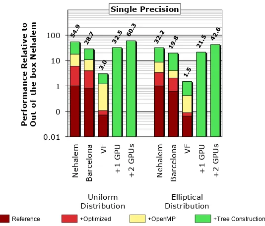
com-54.9 28.7
3.0
32.5 60.3 32.2 19.8
1.5 21.5
42.6
0.01 0 1 10 100
Ne
h
al
em
B
ar
ce
lo
n
a
VF
+
1
G
PU
+
2
G
PU
s
Ne
h
al
em
B
ar
ce
lo
n
a
VF
+
1
G
PU
+
2
G
PU
s
Uniform
Distribution Distribution Elliptical
P
e
rf
o
rm
an
ce
R
e
lat
iv
e
t
o
O
u
t-o
f-t
h
e
-b
o
x
N
e
h
al
e
m
Single Precision
Reference +Optimized +OpenMP +Tree Construction Amortized
Energy assuming CPU consumes no power
Figure 3: Cross-platform comparison of the fast multipole method. All performance is shown relative to an “out-of-the-box” 1-core Nehalem implementation; each bar is labeled by this speedup. VF = Sun’s Victoria Falls multithreaded processor. Note: Figure also appears elsewhere [4].
pared to a single CPU core [8]. As Figure 3 shows, our own GPU implementation did in fact yield this range of speedups compared to a baseline code on a single Ne-halem core [11]. However, we also found that explicit parallelization and tuning of the multicore CPU imple-mentation could yield an impleimple-mentation on Nehalem that nearly matched the dual-GPU code, within about 10%. Like both of the previous computation classes, the same issues arise: (a) there is overhead from necessary GPU-specific data structure reorganization and host-to-GPU copies; and (b) variable workloads, which results in abundant but irregular parallelism as well as sufficiently irregular memory access patterns.
5
Concluding Remarks
The intent of this paper is to consider much of the recent work on GPU acceleration and ask for CPU comparisons in more realistic application contexts. Such comparisons are critical for applications like the ones we consider here, which lie somewhere between computations that are completely regular (e.g., dense matrix multiply) and those that are “wildly” irregular (tree-, linked-list, and graph-intensive computations). For our computations, adding a GPU to a CPU-based system is like adding roughly one or two sockets of performance.
This performance boost is not insignificant, and sug-gests the fruitfulness of hybrid CPU/GPU implementa-tions, which we are in fact pursuing. However, our
obser-vations also raise broader questions about the boundary between when a GPU outperforms a CPU, and whether a productivity loss (if any) of tuning specifically for a GPU is outweighed by the performance gained.
Acknowledgments
We thank Scott Klasky for (indirectly) posing the initial question considered in Section 1. We thank George Biros for productive discussions about applications, and Hye-soon Kim and Nitin Arora for those about GPUs. We also thank Agata Rozga for suggesting the use of the term “wet blanket.”
This work was supported in part by the National Sci-ence Foundation (NSF) under award number 0833136, NSF CAREER award number 0953100, NSF TeraGrid allocation CCR-090024, joint NSF 0903447 and Semi-conductor Research Corporation (SRC) Award 1981, a Raytheon Faculty Fellowship, and grants from the De-fense Advanced Research Projects Agency (DARPA) and Intel Corporation. Any opinions, findings and con-clusions or recommendations expressed in this material are those of the authors and do not necessarily reflect those of NSF, SRC, DARPA, or Intel.
References
Conf. Parallel Processing (ICPP), Vienna, Austria, September 2009.
[2] N. Bell and M. Garland. Implementing a sparse matrix-vector multiplication on throughput-oriented processors. InProc. ACM/IEEE Conf. Su-percomputing (SC), Portland, OR, USA, November 2009.
[3] C. Cecka, A. J. Lew, and E. Darve. Assembly of fi-nite element methods on graphics processors.Int’l. J. Numerical Methods in Engineering, 2009.
[4] A. Chandramowlishwaran, S. Williams, L. Oliker, I. Lashuk, G. Biros, and R. Vuduc. Optimizing and tuning the fast multipole method for state-of-the-art multicore architectures. InProc. IEEE Int’l. Paral-lel and Distributed Processing Symp. (IPDPS), At-lanta, GA, USA, April 2010.
[5] J. W. Choi, A. Singh, and R. W. Vuduc. Model-driven autotuning of sparse matrix-vector multi-ply on GPUs. In Proc. ACM SIGPLAN Symp. Principles and Practice of Parallel Programming (PPoPP), Bangalore, India, January 2010.
[6] J. W. Demmel. Applied Numerical Linear Algebra. SIAM, Philadelphia, PA, USA, 1997.
[7] L. Greengard and V. Rokhlin. A fast algorithm for particle simulations. J. Comp. Phys., 73:325–348, 1987.
[8] N. A. Gumerov and R. Duraiswami. Fast multipole methods on graphics processors. J. Comp. Phys., 227:8290–8313, 2008.
[9] M. E. Guney. High-performance direct solution of finite-element problems on multi-core processors. PhD thesis, Georgia Institute of Technology, At-lanta, GA, USA, May 2010.
[10] E.-J. Im, K. Yelick, and R. Vuduc. SPARSITY: Optimization framework for sparse matrix kernels.
Int’l. J. High Performance Computing Applications (IJHPCA), 18(1):135–158, February 2004.
[11] I. Lashuk, A. Chandramowlishwaran, H. Langston, T.-A. Nguyen, R. Sampath, A. Shringarpure, R. Vuduc, L. Ying, D. Zorin, and G. Biros. A mas-sively parallel adaptive fast multipole method on heterogeneous architectures. InProc. ACM/IEEE Conf. Supercomputing (SC), Portland, OR, USA, November 2009.
[12] NVIDIA. NVIDIA’s next generation CUDA compute architecture: FermiTM, v1.1. Whitepa-per (electronic), September 2009. http://
www.nvidia.com/content/PDF/fermi_ white_papers/NVIDIA_Fermi_Compute_
Architecture_Whitepaper.pdf.
[13] D. A. Patterson. The top 10 innova-tions in the new NVIDIA Fermi archi-tecture, and the top 3 next challenges.
http://www.nvidia.com/content/PDF/ fermi_white_papers/D.Patterson_
Top10InnovationsInNVIDIAFermi.pdf,
September 2009.
[14] R. Vuduc, J. W. Demmel, and K. A. Yelick. OSKI: A library of automatically tuned sparse matrix ker-nels. InProc. SciDAC, J. Physics: Conf. Ser., vol-ume 16, pages 521–530, 2005.
[15] S. Williams, N. Bell, J. Choi, M. Garland, L. Oliker, and R. Vuduc. Sparse matrix vector multiplication on multicore and accelerator systems. In J. Don-garra, D. A. Bader, and J. Kurzak, editors,Scientific Computing with Multicore Processors and Acceler-ators. CRC Press, 2010.
[16] S. Williams, R. Vuduc, L. Oliker, J. Shalf, K. Yelick, and J. Demmel. Optimizing sparse matrix-vector multiply on emerging multi-core platforms. Parallel Computing (ParCo), 35(3):178–194, March 2009. Extends conference version: http://dx.doi.org/10.1145/
1362622.1362674.
[17] L. Ying, G. Biros, D. Zorin, and H. Langston. A new parallel kernel-independent fast multipole method. InProc. ACM/IEEE Conf. Supercomput-ing (SC), Phoenix, AZ, USA, November 2003.