This is anearly accessversion of
Steinert-Threlkeld, Shane & Jakub Szymanik.2019. Learnability and semantic universals.Semantics and Pragmatics 12(4).https://doi.org/10.3765/sp. 12.4.
This version will be replaced with the final typeset version in due course. Note that page numbers will change, so cite with caution.
early access
Learnability and semantic universals
*Shane Steinert-Threlkeld
Department of Linguistics University of Washington
Jakub Szymanik
Institute for Logic, Language and Computation
Universiteit van Amsterdam
Forthcoming inSemantics & Pragmatics.
Abstract One of the great successes of the application of generalized quantifiers to natural language has been the ability to formulate robust semantic universals. When such a universal is attested, the question arises as to the source of the universal. In this paper, we explore the hypothesis that many semantic universals arise because expressions satisfying the universal are easier to learn than those that do not. While the idea that learnability explains universals is not new, explicit accounts of learning that can make good on this hypothesis are few and far between. We propose a model of learning — back-propagation through a recurrent neural network — which can make good on this promise. In particular, we discuss the universals of monotonicity, quantity, and conservativity and perform computational experiments of training such a network to learn to verify quantifiers. Our results are able to explain monotonicity and quantity quite well. We suggest that conservativity may have a different source than the other universals.
Keywords:semantic universals, generalized quantifiers, monotonicity, quantity, conserva-tivity, neural networks, learnability
early
access
1 Introduction
At first glance, the natural languages of the world exhibit tremendous differences amongst themselves. After all, learning a second language as an adult is not an easy task. Yet, early in one’s linguistics education, one learns that languages do share tremendous amounts of structure and that the differences can be described, circumscribed, and analyzed. Thus arises one of the central questions in linguistic theory: What is the range of variation in human languages? That is: which out of all of the logically possible languages that humans could speak, do they in fact speak? A limitation on the range of possible variation will be a property that all (or, at least almost all) languages share. Such a property will be a linguisticuniversal.
Universals have been discovered at all levels of linguistic analysis. At the phono-logical level, all languages have consonants and vowels. More robustly, one can say that all languages have at least one unrounded vowel and at least one back vowel.1 At the syntactic level, all languages have verbs and nouns.2 Slightly more controversially, generative grammar as an enterprise can be seen as systematically developing syntactic universals. For example, the basic claim that grammatical rules are structure-dependent3 is a syntactic universal. At the semantic level, it has been proposed that all languages which have shape adjectives also have color and size adjectives.4 Closer to the topic of the present paper is the claim that all languages have syntactic constituents (Noun Phrases) whose semantic function is to express generalized quantifiers.5
Whenever a universal is attested, it is natural to ask for an explanation of its source.Whydoes the universal hold? While significant differences as to the type of answer to this question arise in the phonological and syntactic domains, many theo-rists search forcognitiveexplanations of semantic universals. Such an explanation would locate the existence of a semantic universal in a feature of human conceptual apparatus with which semantics must interface.
The present paper develops the hypothesis that semantic universals are to be explained in terms oflearnability, at least in the domain of quantifiers. We focus on
1 SeeHyman 2008for a thorough discussion of phonological universals, including these two, where they are called “Vocalic Universal #3” and “Vocalic Universal #4” on p. 98.
2 SeeCroft 1990.Newmeyer(2008) calls for hesitation on positing universals about syntactic categories.
Hengeveld et al.(2004) discuss examples of languages that seem not to make the distinction. 3Chomsky 1965, and many others.
4 SeeDixon 1977for that universal.von Fintel & Matthewson(2008) provide an overview of semantic universals.
early
access
quantifiers simply because this is the area where the largest number of substantial semantic universals have been posited. In developing this hypothesis, we do not claim that learnability will be the only source of semantic universals. For example, communicative need may play a key role in some explanations. Rather, we want to explore how far the learnability hypothesis can be pushed in this domain.
In the literature, there are at least two forms that the learnability argument takes. The first one focuses on the fact that a universal can restrict the hypothesis space for a hypothetical learner of a semantic system.6 Because a universal greatly shrinks the space of possible quantifier meanings, the learner does not have to explore as much. This makes it is easier7 to learn these meanings. Seen this way, this learnability argument mirrors at the semantic level Chomsky’s poverty of the stimulus argument for universal grammar.8
At a certain level, this first argument has to be correct: learning in a smaller hypothesis space will invariably be easier than learning in a larger one. Nevertheless, one should not overstate its conclusions, for two reasons. Firstly, it could be that the benefit to learning from moving to a smaller space is quite negligible.Piantadosi (2013), in a paper where he explores Bayesian learning of quantifiers, puts the point very eloquently:
Likely, the unrestricted space has many hypotheses which are so implausible, they can be ignored quickly and do not affect learning. The hard part of learning, may be choosing between the plausible competitor meanings, not in weeding out a large space of potential meanings. (p. 22)
Secondly, and more fundamentally, this form of argument can only explain why there are universals at all, but notwhichuniversals one observes. Any proposed se-mantic universal has the benefit of decreasing the hypothesis space for the language learner. Because of that, this argument cannot distinguish between competing univer-sals and so cannot explain the exact pattern of univeruniver-sals that are attested. The most that could be gleaned from this line of reasoning would be that one should search for
strongeruniversals, since they consist in larger reductions of the hypothesis space and so presumably provide a bigger benefit to learning.
6Barwise & Cooper (1981),Keenan & Stavi(1986),Szabolcsi (2010) all present a form of this argument.
7 Or, in the most extreme version: possible in the first place.
8 The term is coined inChomsky 1980, though the argument has appeared in many places in his work. SeePullum & Scholz 2002for an overview and assessment. BothMay(1991) andPartee
early
access
The second form of the learnability argument runs as follows: semantic universals hold because expressions satisfying the universal areeasierto learn than those that do not.9 Implicit here is a certain linking hypothesis: meanings that are easier to learn are more likely to be lexicalized. While this paper will not address this hypothesis, it is intuitively plausible: languages have words for meanings that are easier to learn and use compositional methods to express more difficult-to-acquire meanings. As it presently stands, however, this second argument has a major lacuna. For no semantic universals has the argument been fully developed. In order to be more than a suggestion, one cannot simply suggest that expressions satisfying a universal are easier to learn but must actually demonstrate that this is so. This can be seen as a challenge.
CHALLENGE: For the semantic universal(s) of choice, provide a model of learning
on which expressions satisfying the universal are easier to learn than others.
The present paper aims to meet the CHALLENGE. In particular, we will focus on three universals in the domain of quantifiers: monotonicity, quantity, and conserva-tivity. We propose a model of quantifier learning by showing how to train a certain kind of recurrent neural network to learn to verify quantified sentences. Computer simulations yield promising initial results. For both the monotonicity and quantity universals, we ran two experiments and found in each that a quantifier satisfying the universal is indeed easier to learn by this model than one that does not. The case of conservativity is more complicated: for reasons to be discussed later, we did not expect our learning model to be sensitive to conservativity. Still, we ran two experiments as a kind of benchmark. As expected, in both experiments, a conserva-tive and non-conservaconserva-tive quantifier are indistinguishable in terms of learnability. Against this backdrop, we argue that this might not be a problem since that universal arguably has a different source.10
The paper is structured as follows. Section2 presents a brief introduction to generalized quantifiers and explains the three universals that we will study. Section3 presents the model of learning — backpropogation-through-time in a recurrent neural network — that we will apply to quantifiers. In Section4, we present experiments where we apply the model to each of the universals, with mostly positive results. We provide a general discussion of the results and possible objections in Section5. In particular, we argue that learnability by a recurrent neural network can be viewed
9Peters & Westerståhl(2006) (p. 173) allude to this argument for one of the quantifier universals to be discussed later.
early
access
as an operationalization of a general notion of semantic complexity. Finally, we conclude in Section6by recording some future directions of research.
2 Quantifier universals
The universals that we focus on have to do with quantifiers, which are the semantic objects expressed bydeterminers. A determiner is an expression taking a common noun as an argument and generating a Noun Phrase. We will assume a division of the determiners in to two classes: simple and complex. Examples of simple determiners areall, some, no, few, most, five. Examples of complex determiners areall but five, fewer than three, at least eight or fewer than five. Note that we do not at present provide a full account of exactly what the distinction amounts to. For example, while being monomorphemic certainly suffices for being simple, we leave it open that some determiners that are not monomorphemic will still count as simple.11
As a first approximation, and following the influentialBarwise & Cooper 1981, we assume that determiners denote typeh1,1igeneralized quantifiers. These can be thought of as being relations between two subsets of a given domain of discourse. For example:
JeveryK={hM,A,Bi: A⊆B} Jat_most_3K={hM,A,Bi: |A∩B| ≤3}
JmostK={hM,A,Bi: |A∩B|>|A\B|}
Before proceeding, a few small notes on terminology. As a shorthand, we will say that a determiner has a certain semantic property to mean that the quantifier that the determiner denotes has that property. Sometimes, for a determiner likeevery, we will write everyas a shorthand forJeveryK. We will useQand its ilk as variables over quantifiers. Because quantifiers are viewed as set-theoretic objects, we will writeM ∈Qwhen a structure/modelM belongs to a quantifier.12 In other words, when a sentenceDet N VPis true when interpreted in a model M, we will write hM,JNK,JVPKi ∈Det. In the remainder of this section, we introduce three prominent semantic universals about quantifiers.
2.1 Monotonicity
To motivate our first universal, consider the following sentences.
11 Arguably,mostis not monomorphemic. SeeHackl 2009,Kotek et al. 2011a,b,Solt 2016. Moreover, some argue that a much wider class, includingnoandfew, are also not monomorphemic. But these arguably should count as simple for the purpose of formulating semantic universals.
early
access
(1) a. Many French people smoke cigarettes. b. Many French people smoke.
It is clear that (1a) entails (1b): the former cannot be true without the latter being true. Similarly, this entailment does not depend on the choice of the restrictor —French people— or scopes —smoke cigarettesandsmoke— so long as the latter scope is strictly more general than the former. Moreover, competent speakers of English recognize this fact easily. What speakers thereby implicitly know is thatmanyis upward monotone:
(2) Qisupward monotoneif and only if wheneverhM,A,Bi ∈QandB⊆B0, then hM,A,B0i ∈Q.
By contrast, the pattern seems to reverse if we replacemanywithfew, as seen in the following examples.
(3) a. Few French people smoke cigarettes. b. Few French people smoke.
Here, (3b) entails (3a). This is the reverse of the previous case: now, truth is preserved when we move from a more general scope to a more specific scope. In this case, we say thatfewis downward monotone:
(4) Qisdownward monotoneif and only if wheneverhM,A,Bi ∈QandB⊇B0, thenhM,A,B0i ∈Q.
Finally, a determiner ismonotone if and only if it is either upward or downward monotone. The reader can verify that all of the simple determiners mentioned at the beginning of the section are monotone. This appears to be no accident of our choice of English or of that particular list of simple determiners.Barwise & Cooper(1981) proposed the following semantic universal.
MONOTONICITYUNIVERSAL: All simple determiners are monotone.
This universal rules out quantifiers such as an even number of and at least 6 or at most 2: increasing or decreasing the setBcan cause the cardinality ofA∩Bto change in a way that flips the truth value of sentences with those determiners, so they are not monotone. The claim then is that no simple determiner in any natural language denotes those quantifiers.
2.2 Quantity
early
access
the formDet A Bshould not depend on the identity of any particularAorB, nor on the manner of presentation of those sets. We will build up to the next universal in stages, beginning with an idea borrowed from discussions of logical constants. A
permutationof a set is a bijection from that set to itself. Permutations can be lifted from sets to models with that set as its domain of discourse in a natural way. We can then say what it is for a quantifier to be logical.
(5) Q is logical if and only if for all sets M and permutations π :M →M, hM,A,Bi ∈Qif and only ifhπ(M),π(A),π(B)i ∈Q.
In their seminal paper,Keenan & Stavi(1986) propose the universal that “Monomor-phemic dets are logical” (p. 311). This rules out expressions such as possessives (e.g.Susan’s) whose truth does depend on a particular element of the model and so might not be preserved when the elements are permuted. Of course, possessives are not monomorphemic; the universal claims that no monomorphemic determiner could have the same meaning as a possessive likeSusan’s.13
A slightly stronger universal than logicality appears to hold. It replaces permutation-invariance with isomorphism-permutation-invariance. Anisomorphismbetween two models is a bijection between their underlying sets that preserves the additional structure of the model. In the case of models of the formhM,A,Bi, this means thatAgets mapped toA0andBtoB0.
(6) Q is isomorphism-invariant if and only if: if hM,A,Bi ∼=hM0,A0,B0i, then hM,A,Bi ∈Qif and only ifhM0,A0,B0i ∈Q.14
Peters & Westerståhl (2006) formulate and defend the universal that all simple determiners are isomorphism-invariant.15 In other words, they endorse the following universal.16
QUANTITY UNIVERSAL: All simple determiners are isomorphism-invariant.
To understand what quantifiers this universal rules out as the denotations of simple determiners, note the following fact:hM,A,Bi ∼=hM0,A0,B0iif and only if the four setsA∩B,A\B,B\A, andM\(A∪B)have the same cardinality as their primed counterparts.17 So the QUANTITYUNIVERSALsays that the truth value of a
13 SeePeters & Westerståhl 2013for a thorough analysis of possessives.
14 Generalized quantifier theory, as developed in mathematical logic, generally builds isomorphism-invariance into the definition of a quantifier. SeeMostowski 1957,Lindström 1966for the founding documents of that tradition. For application to natural language, however, we do not impose the requirement but see it as an additional constraint on quantifiers.
15 Their exact wording (p. 330): “All lexical quantifier expressions in natural languages denote ISOM quantifiers.”
early
access
simple sentence of the formDet N VPdepends only on those four quantities. This rules out lexical items from having the same meaning as exceptive phrases likeall . . . except engineersin sentences such as:
(7) All students except engineers must take a creative writing class.
In particular, the truth of this sentence depends on membership in a fixed set of engineers, and not merely the sizes of the sets built out of the students and those taking a creative writing class.
Additionally ruled out as candidate meanings of simple determiners are quan-tifiers that depend on themanner of presentationof the restrictor and scope. For example, consider the following.
(8) The first three students to solve the problem will get extra credit. (9) Every other house on that block is vacant.
The truth of both (8) and (9) depends on the order in which elements of the re-strictor —studentsandhouse on that block, respectively — are inspected. It seems that no language has a lexical itemfthreewhich has the meaning ofthe first three
in (8).18 Similarly, one can imagine other sentences whose truth depends on the spatial arrangement of the restrictor. All such expressions are ruled out as possible determiners by the QUANTITY UNIVERSAL.
2.3 Conservativity
Our final universal — arguably the most widely discussed of the three — captures the intuition that the restrictor genuinely restricts what a sentence talks about. That is, sentences of the formDet N VPare in some sense about theNs and nothing else. That this universal holds can be observed by noting the felt equivalence between the following pairs of sentences.
(10) a. Every student passed.
b. Every student is a student who passed. (11) a. Most Amsterdammers ride a bicycle to work.
b. Most Amsterdammers are Amsterdammers who ride a bicycle to work.
The formal concept at play here has been called conservativity.
(12) Qisconservativeif and only ifhM,A,Bi ∈Qif and only ifhM,A,A∩Bi ∈Q.
early
access
Barwise & Cooper(1981) formulated and defended the following universal.19
CONSERVATIVITY UNIVERSAL: All simple determiners are conservative.20
This universal rules out quantifiers that depend on other portions of the model besides
A, such asB\A. As an example, there is no determinerequiin any language such that the following two sentences are equivalent in meaning.
(13) a. Equi students are at the park.
b. The number of students is the same as the number of people at the park.
This concludes the presentation of the semantic universals to be studied here. Because we primarily focus on the explanation/source of semantic universals, we do not present a detailed defense of each universal. Rather, we assume that the universals hold and attempt to explain why they do in terms of learnability. That being said, we know of virtually no counter-examples to the three universals being studied.21
3 The learning model
Recall that our CHALLENGEwas to provide a model of learning on which expressions
satisfying semantic universals were easier to learn than those that do not. Having now explained three such universals in the domain of quantifiers, we develop model of learning quantifiers. In the next section, we present experiments showing that this model can meet the CHALLENGE.
The basic idea will be to train aneural networkto learn how to verify and falsify quantified sentences. A neural network is a computational device modeled after the methods of computation and communication in biological nervous systems.22 Such
19 Because the termconservativewas not introduced untilKeenan & Stavi 1986, the original formulation was in terms of a quantifierliving ona witness set. We follow the norm of formulating in terms of conservativity for concision.
20 In fact, conservativity often is a claim about all determiners, not just the simple ones. This claim sits well with the view we defend in Section4.3that this universal is not a constraint on the lexicon but arises from the workings of the syntax-semantics interface.
21 Most prominently, ‘only’ and the reverse proportional reading of ‘many’ (first observed inWesterståhl 1985) have been claimed to be counter-examples to CONSERVATIVITY. One can argue that neither is a determiner: the former is an adverb (von Fintel 1997) and the latter a gradable adjective (Romero 2015). Or one can observe that they are ‘conservative on their second argument’ and attempt to assimilate this to standard conservativity. Seevon Fintel & Keenan 2018for a recent discussion and references.
22 SeeRumelhart et al. 1986a,bfor an overview of early pioneering work applying neural networks to human cognition. For modern overviews of this area of research, we recommendNielsen 2015,
early
access
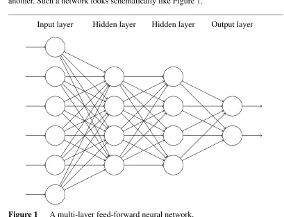
a network consists of a number ofnodes, which are arranged sequentially inlayers. Activation — a numerical quantity — travels through the layers because nodes in one layer are connected to those in the subsequent one. The connections between nodes can have different weights, reflecting how important the activation in one node is to another. Such a network looks schematically like Figure1.
Input layer Hidden layer Hidden layer Output layer
Figure 1 A multi-layer feed-forward neural network.
The first layer is called theinput layer. The final layer is called theoutput layer. If the input layer hasnnodes and the output layer hasmnodes, then the network computes a function fromRntoRm. The layers — if there are any — in between the input and output layers are called hidden layers. Computation works as follows: each node computes a weighted combination of the activations of the nodes that connect to it and then applies a nonlinearity. Somewhat more concretely, for a non-input layerl, we have that
(14) ~al= fWl·~al−1+~bl
where~al is the vector of activations in layerl,Wl is a matrix containing theweights
early
access
l−1 to node jin layerl),~bl is a vector of biases, and f is some non-linear function applied point-wise.23
Such a network learns to approximate a given function by gradually updating the weights and biases in a way that it moves closer to the given function. Formally, this is done by (stochastic)gradient descent. Letting~θ denote a long vector containing all of the parameters of the network (i.e. all the weights and biases), we can think of the network as computing a function of these parameters and the input, which we will denoteNN(~θ,~x), where~xis an input. The learning will be supervised: we have a set of data points~xi,~yi
i∈I, indexed by a finite setI, which (partially) capture the given function’s input-output relationship. We assume that there is a total loss function, which is the mean of a ‘local’ error function`.`is defined onRm×Rm, and measures how close the network’s output is to the true output.
(15) L=|1I|∑i`(NN(~θ,~xi),~yi)
Gradient descent works by consideringLas a function of~θ, and then moving around that space towards lower and lower values ofL. Formally, at iterationt of training, the parameters of the network are updated by
(16) ~θt+1←~θt−α∇~θL
whereα is a learning parameter. The gradient∇~
θLcan be computed by the famous
backpropagationalgorithm. Intuitively, a forward pass through the network generates a guess, after which an error`is calculated. This error can be sent in a backward pass through the network to compute the partial derivative with respect to each parameter.
In practice, more complicated update rules than (16) — with learning rates that are not constant — are deployed. Similarly, stochastic gradient descent improves on this by updating after a mini-batch of data points (as small as one example) is processed, instead of only updating after all of the data have been processed. Conceptually, however, the algorithms work the same way: the weights and biases of the network are updated in such a way that loss is reduced, moving the network’s function closer to the true function.
To train a neural network to learn the meanings of quantifiers, we will have it learn to doquantifier sentence verification. That is, we want the input to the network to be a pair hM,Qiof a model and a quantifier expression, and the network will output a 1 or a 0 corresponding to whether M ∈Q or not. More precisely, the network will output a probability: how strongly the network ‘believes’ thatM ∈Q.
Two features of this task require moving to a model slightly richer than a standard feed-forward neural network as just described. Firstly, the models belonging to a quantifier can come in many different sizes, but these neural networks require a
23 Common choices here are the sigmoidσ(x) = 1
1+e−x and hypertangent tanh(x) =e x−e−x
early
access
fixed-length input. In practice, one often extracts featuresfrom an input, so that variable-sized inputs get mapped to a fixed-sized representation. We do not, however, want to pre-select the features of a model that will be relevant to the quantifier verification task, preferring to give the network the raw model. Secondly, to model quantifiers likefirst threethat fail the QUANTITYUNIVERSAL, we want the model to be presentedsequentiallyto the network, so that it can be sensitive to the order of presentation of objects.
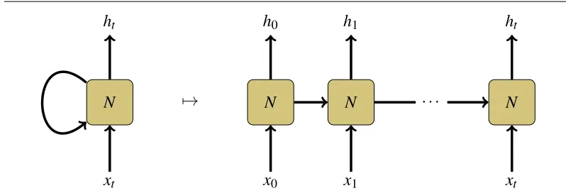
So-calledrecurrent neural networksovercome both of these limitations. The key innovation in these networks is that they have ‘loops’: as they process a sequential input, they maintain a state that gets passed on to the next step.24 Networks of this type are trained by a method called Backpropagation-Through-Time.25 Essentially, the loops in the network are ‘unfolded’ for as many steps as in the input sequence, and standard backpropagation is used to calculate the gradients. Figure2depicts the architecture and this unraveling schematically. In this Figure and in what follows, we omit the use of arrows to denote vectors in order to improve readability.
N
xt
ht
7→ N
x0
h0
N
x1
h1
N
xt
ht
· · ·
Figure 2 A recurrent neural network (RNN), unrolled as in Backpropagation-Through-Time. Thexiare the input sequence of vectors, and thehiare output vectors. At time-step i, an RNN receives both xi and hi−1 as inputs. (At the first time-step, someh0 must be fed into the network. Typically, this will be all zeros or a random vector.) The boxedN repre-sents some mathematical function, usually a kind of neural network.
The particular form of RNN that we will use is called along short-term memory (LSTM)network.26 While these were introduced to solve a technical problem in
24 For early applications, seeJordan 1986,Elman 1990,Bengio 1991. 25 SeeWerbos 1988for an early version of the algorithm.
early
access
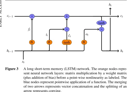
training RNNs,27 they also admit of an intuitive interpretation. As the network processes a sequence, it maintains a statect. At itemt in the sequence, the network chooses which bits of the cell to forget, and which bits of the input to write to the cell. In this way, the network maintains a form of memory as it processes a sequence. Mathematically, the network computes the following function, depicted schematically in Figure3, and subsequently explained intuitively.
(17) LSTM computation:
ft =σ
Wf·ht−1xt+bf
it =σ Wi·ht−1xt+bi
ˆ
ct =tanh(Wc·ht−1xt+bc)
ct = ftct−1+itcˆt
ot =σ(Wo·ht−1xt+bo)
ht =ottanh(ct)
In the equations above,denotes component-wise multiplication, andht−1xt repre-sents vector concatenation. Note that the computation of f,i,cˆ,oare instances of the basic neural network layer activation computation from equation (14), withht−1xt
as the ‘previous activation’.
The equations ft andit should be thought of as forget and input gates, respec-tively. Consider ft. It will be a vector of the same number of dimensions asct. The sigmoid activation function used outputs values between 0 and 1. The value of ft
in dimension jcan be thought of as how strongly to ‘remember’ element j of the state vectorct−1. This is due to the element-wise multiplication of ft andct−1 in the calculation of ct. For instance, if element j of ft is 0, then the corresponding element ofct−1will be entirely erased. The input gateitworks similarly, though it interacts not directly withct−1, but with a set of ‘candidate’ values ˆct for the next state vectorct. Finally, the equation forct encapsulates the idea that values of the state are forgotten according to ftand new ones are written according toit. One last output gateot filters which components of the cellct to output at each time step.
Before proceeding, we make two remarks motivating our choice of LSTM net-works. Firstly, these networks have become the gold standard type of neural network for processing sequential data. They have been crucial components in models that have achieved remarkable results in tasks like language modeling,28 image and
27 The so-called problem of vanishing and exploding gradients: the unrolling used in BPTT tends to produce gradients that either become very close to zero or very large.
early
access
σ σ tanh σ
×
×
+
tanh
×
ht−1
ct−1 ct
xt
ft
it cˆt ot
ht ht
Figure 3 A long short-term memory (LSTM) network. The orange nodes repre-sent neural network layers: matrix multiplication by a weight matrix (plus addition of bias) before a point-wise nonlinearity as labeled. The blue nodes represent pointwise application of a function. The merging of two arrows represents vector concatenation and the splitting of an arrow represents copying.
video captioning,29 and machine translation.30 To that end, we have not tailor-made a network architecture to our task, but grabbed one off-the-shelf and applied it to the task of learning quantifiers. Secondly, recent work in neuroscience shows that gating mechanisms not unlike those that regulate the flow of information in an LSTM (e.g. the forget and input gates) underly the operation of working memory in humans.31 These two factors make our choice of network model extremely natural and well-suited to the task of addressing the CHALLENGE: the model appears to be
domain-general and biologically plausible.
Here is how we will apply an LSTM to the task of verifying a quantifier. We want its input to be a sequence, representing a model, together with a quantifier, and its output to be a guess at the truth-value. Thus, it is asequence classification
task.32 The relevant truth-value to be guessed is for a sentence of the form ‘Q A
29Xu et al. 2015,Donahue et al. 2017
30Sutskever et al. 2014,Wu et al. 2016
31McNab & Klingberg 2008,Gisiger & Boukadoum 2011
early
access
B’. Because our focus is on learning the meaning of the quantifier and not on any syntactic parsing, we take theAandBto be schematic and present the model with objects labeled for their membership in those sets.
The zones of a model —A∩B,A\B,B\A,M\(A∪B)— will be encoded as one-hot vectors. For example, an element ofA∩Bwill be encoded as1 0 0 0. We assume the models are enumerated, and run through the enumeration, generating a sequence of vectors. Finally, each quantifier is also labeled with a one-hot vector, in as many dimensions as there are quantifiers. The vector for the quantifier is concatenated to each element’s vector. One can think of this in the following way: as the network processes the model sequentially, it always has access to the sentence that it’s attempting to verify in much the same way as human participants often do in sentence-verification experiments. This should make the learning task slightly easier, since the network does not have to remember what quantifier it is verifying. In (18), we provide a detailed example of this encoding.
(18) Encoding a model as a sequence for the LSTM.
∈A? ∈B? xi
o1 X X
1 0 0 0 0 1
o2 X x
0 1 0 0 0 1
o3 x X
0 0 1 0 0 1
o4 X X 1 0 0 0 0 1
o5 x x
0 0 0 1 0 1
In the above table, theoi are the five objects of a model, presented in that order. The next two columns indicate whether each object belongs to the set
A(the restrictor) orB(the nuclear scope), respectively. Finally, thexicolumn represents the input at stepito the LSTM for this example.
In this example, we assume that the network is being trained on two quanti-fiers —every andsome— and that they are ‘ordered’ in that way. The final two dimensions of eachxiencode that the desired/intended output is the truth value of ‘someAis aB’. When it is being asked to output the truth value of ‘everyAis aB’, the final two dimensions will be1 0for eachxi.
Finally, the true labelyfor this example will be1 0, because the sentence is indeed True. The truth-value False is represented by the vector0 1.
early
access
After the LSTM processes the sequence corresponding to a model and quanti-fier, the final output is passed to a one-layer feed-forward neural network with two outputs, corresponding to True and False. This output layer has a softmax activation function, so that the resulting activations are probabilities.33 Full details of the net-work architecture and the data generation process will be described in the following section.
This choice of input captures some necessary features for addressing the CHAL
-LENGE. If, for instance, we encoded models by the cardinalities of the four respective sets, we would not be able to represent quantifiers that do not satisfy QUANTITY.
Similarly, if we did not represent all four sets but only the setsA∩BandA\B, we would not be able to represent non-conservative quantifiers.34
To complete the description of the learning model, we must specify what loss function we will be minimizing. In tasks like ours where the output is a probability distribution, the standard choice is cross-entropy. This function can be seen as capturing the ‘distance’ between two probability distributions. Or, since it’s not symmetric, the amount of ‘work’ that one would have to do to transform a given distribution into a target one. For discrete distributions, the general form is:
(19) E(p,q) =−∑mi=1p(xi)lnq(xi)
In our case, this takes on a particularly simple form. This is because the target distribution pcomes from our training data, and so assigns all of the probability to the correct truth-value, and none elsewhere. Thus, fory∈ {0,1}being the correct truth-value, our local error function will be:
(20) `(NN(θ,x),y) =−ln(NN(θ,x)y)
This makes good intuitive sense. Becauseyis the correct truth-value,NN(θ,x)yis the probability that the network assigns to the correct truth-value. When this probability equals 1 (i.e. when the network completely correctly guesses the right truth-value), then ` is 0. And as this probability gets farther and farther away from 1, the loss increases. Plugging this local error function into a gradient descent algorithm, then, means that the network will learn to assign higher and higher probability to the correct truth-value.
33 Withva vector, softmax(v)i=evi/∑jevj. We could use just one node, since the guess is a probability, but having two outputs allows for easier generalization to other classification tasks.
early
access
4 Experiments
We are now in a position to directly address the CHALLENGE: we have three proposed
semantic universals about quantifiers and a model of learning quantifiers. We can thus ask, for each of the universals, the following question: are expressions satisfying the universal easier to learn (by an LSTM) than those that do not? In this section, we present three experiments, one for each universal. Because all experiments shared the same methodology, we first describe the methods. All code for running the simu-lations and the data generated are available at http://github.com/shanest/quantifier-rnn-learning.
For each universal, we do the following: choose a pair of quantifiers, one sat-isfying the universal and one not satsat-isfying it. We then run some number of trials of training an LSTM to learn those two quantifiers. Multiple trials are needed for a robustness check since the learning is a stochastic process.35 For each trial, we measure how long it took the network to converge for each quantifier, and compare the two, where convergence means having reached and maintained a suitably high threshold of accuracy.36 To meet the CHALLENGE, we hope that the networks systematically converge earlier for the quantifier satisfying the universal.
More concretely, Algorithm 1 below depicts our data generation algorithm. Essentially, a quantifier is drawn at random, and a sequence corresponding to a model of a randomly-chosen size is also generated. We then add the corresponding data point to the data set, avoiding duplicates. Finally, we shuffle the data, and balance it so that every quantifier/truth-value pair has the same number of data points. The balancing is done by under-sampling to the smallest class.37 We then split the generated data into a training set and a test set. In all of our experiments, the split was 70%/30%. The algorithm has three parameters: the maximum length of a model, the number of data points to generate, and a set of quantifiers. For all experiments, the maximum length was 20. The other two parameters varied by experiment and so will be reported for each. We varied the total number of data points generated for the following reason: at the end, the data is balanced so that each quantifier/truth-value pair has the same number of data points, so that the network does not simply learn a bias in the data. We performed this balancing by under-sampling, so that each pair ended up with the same number of data points as the least-frequent quantifier/truth-value pair. Because different quantifiers have a different distribution of truth-values across the space of models (for example,mostis true roughly half the time, whileallis very rarely true), we varied the total number of
35 Initialization of the LSTM state and of the weights are random, as is the data generation algorithm, both in exactly which input sequences get generated and the order they are presented to the network. 36 We state our precise measure of convergence below.
early
access
Algorithm 1Data Generation Algorithm
Inputs:max_len,num_data,quants
data←[]
whilelen(data)<num_datado
ChooseN uniformly at random from between 1 andmax_len ChooseQuniformly at random fromquants
cur_seq←N randomly chosen items from{A∩B,A\B,B\A,M\(A∪B)} ifhQ,cur_seqi∈/datathen
AddhQ,cur_seq,cur_seq∈Q?itodata end if
end while shuffle(data)
balance_by_undersampling(data)
returntrain_split(data),test_split(data)
data points generated so that the resulting number of data points per quantifier/truth-value pair were roughly the same across experiments once the under-sampling was performed.
For each experiment, we ran 30 trials of learning. Our networks consisted of two stacked LSTM cells, each with a hidden state of 12 nodes. We stopped the model when the total loss was below 0.01, total mean accuracy for 100 training mini-batches was over 99%, or 4 epochs have passed,38 whichever came first. We used mini-batches of size 8.39 We used the Adam optimizer40 with learning rate 10−5. All of this was implemented using TensorFlow.41
For analysis, we measured the convergence point for each quantifier: this is the first time step where both the accuracy and the mean accuracy on thetest set from then until the end of the trial were above 95%. To see whether one quantifier systematically converged earlier than the other, we calculated a pairedt-test on the convergence points, which is equivalent to a 1-samplet-test on the differences be-tween the two points. This was chosen because within-trial difference of convergence
38 In machine learning, an epoch is one pass through the entire set of training data. SeeNielsen 2015, ch. 1, for this and other terminology.
39 A mini-batch is how much data is used before updating the network. In standard gradient descent, the batch is the size of the entire training data, i.e. the network only computes gradients and updates after seeing all its data. Because this is costly,stochastic gradient descentuses smaller batches. In general, the smaller the batch-size, the worse the approximation to the total gradient, so the more chaotic learning will be.
40Kingma & Ba 2015
early
access
points is more meaningful than comparisons across trials due to the stochastic nature of the learning process.
4.1 Monotonicity
Our first experiment tested the MONOTONICITY UNIVERSAL. Because a quantifier can be either upward- or downward-monotone, we ran one experiment with an upward monotone quantifier and another one with a downward monotone one. In both cases, we generated 100000 data points.
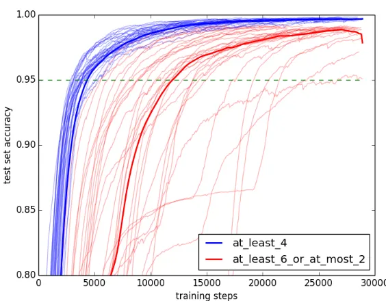
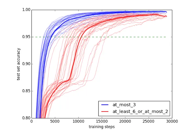
Experiment 1(a) comparedat least 4— an upward-monotone quantifier, meaning |A∩B| ≥4 — with the quantifierat least 6 or at most 2— a non-monotone quantifier meaning|A∩B| ≥6 or|A∩B| ≤2. The learning curves for all of the 30 trials are plotted in Figure4. Qualitatively, it appears thatat least 4regularly converges faster thanat least 6 or at most 2. The statistics confirm this appearance. A pairedt-test of the convergence points found thatat least 4did converge statistically significantly earlier across trials (t =−9.356, p=2.926×10⁻¹⁰).
Figure 4 Experiment 1(a) learning curves. The median at each step is in bold.
early
access
converges faster thanat least 6 or at most 2. The statistics confirm this appear-ance. A pairedt-test of the convergence points found thatat most 3did converge statistically significantly earlier across trials (t=−15.253, p=2.182×10⁻¹⁵).
Figure 5 Experiment 1(b) learning curves. The median at each step is in bold.
These results are very encouraging. Both upward- and downward monotone quantifiers are learned significantly more quickly than a corresponding non-monotone quantifier by an LSTM network. In the context of the present study, this supports the argument that the MONOTONICITYUNIVERSALholds because monotone quantifiers
are easier to learn.
4.2 Quantity
Our second experiment tested the QUANTITY UNIVERSAL. First, we comparedat least 3— a quantifier that is quantitative — with first 3— a quantifier that is not quantitative because it depends on the order in which the restrictor is presented. In this case, we generated 200000 data points. We threw out one trial which failed to reach high enough accuracy for both quantifiers after 4 epochs.42 The learning curves for the remaining 29 trials are plotted in Figure6. Qualitatively, while the
early
access
separation does not look as strong as in Experiments 1(a) and 1(b), it does appear thatat least 3converges faster thanfirst 3. The statistics confirm this appearance. A pairedt-test of the convergence points found thatat least 3did converge statistically significantly earlier across trials (t=−7.549, p=4.032×10⁻⁸).
Figure 6 Experiment 2(a) learning curves. The median at each step is in bold.
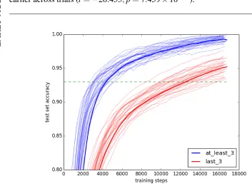
To test the robustness of this result and ensure that it does not reflect a defect in our learning model, we ran a second experiment to test QUANTITY.43 In particular, despite having ‘memory’ in their name, it is known that LSTM networks can in fact have trouble maintaining memory during the course of processing long sequences.44 So it could be what drove the result in Experiment 2(a) was not a general feature of the learning model, but rather a difficulty in maintaining a memory of the early part of the sequence, to whichfirst 3is sensitive. Because of this, we ran a second experiment usinglast 3instead of first 3: this quantifier exhibits the same order-dependency asfirst 3but places less demands on the model’s memory of early parts of a long sequence. The learning curves are plotted in Figure7. Qualitatively, the pattern continues to hold and in fact may be stronger:at least 3appears to converge much faster thanlast 3. The statistics confirm this appearance. A pairedt-test of the
43 We are grateful to an anonymous referee for suggesting this confound and subsequent experiment. 44 This, for instance, partially explains the significant performance boost from reversing the source
early
access
convergence points45 found thatat least 3did converge statistically significantly earlier across trials (t =−26.453,p=7.459×10⁻²²).
Figure 7 Experiment 2(b) learning curves. The median at each step is in bold.
These results, like those before, are encouraging. We have now seen a second universal — the QUANTITY UNIVERSAL— where a quantifier satisfying the uni-versal is learned more easily by an LSTM network than one that does not. That this pattern has been observed for two very prominent universals also lends support to the general argument of which the CHALLENGE is a missing piece: in general, a universal may hold because expressions satisfying it are easier to learn and such expressions are more likely to be lexicalized.
4.3 Conservativity
Our third and final set of experiments focused on the CONSERVATIVITYUNIVER -SAL. Before presenting the results, we note that CONSERVATIVITYappears
some-what different from the previous two universals. While the former two impose robust patterns on the distribution of truth-values for quantified sentences across the space of models, the present universal simply says that one ‘zone’ of a model — namely,
early
access
B\A— is irrelevant. In terms of our learning model, conservativity simply entails that one of the four symbols in the input alphabet will never effect the truth-value (i.e. the classification label); but the patterns of the remaining symbols in the sequences can be of any kind. Because of this difference, there existsprima facie reason to doubt that the model will distinguish conservative from non-conservative quantifiers. We now present two experiments as a kind of ‘sanity check’, exhibiting that this is in fact the case. After so doing, we conclude with a brief discussion of ways the model can be extended to possibly tease apart conservative and non-conservative quantifiers and a positive proposal about the different source of this universal.
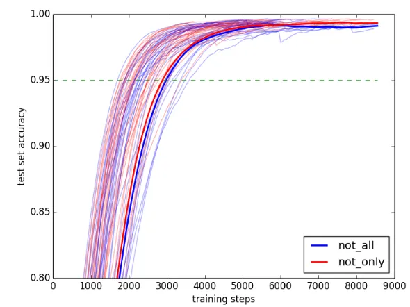
First, we comparednot all— a conservative quantifier meaning thatA6⊆B— with not only— a non-conservative quantifier meaning thatB6⊆A. We chose these two quantifiers followingHunter & Lidz (2013), who taught children to learn a new determiner,gleeborgleeb’. The former —gleeb— meantnot all, while the latter meantnot only. They found that children learned the meaning ofgleebfaster than that ofgleeb’, suggesting that conservative quantifiers are easier for children to learn.
In this experiment, we gathered 300000 data points. The learning curves for all of the 30 trials are plotted in Figure8. Qualitatively, there does not appear to be any significant separation in the learning curves for the two quantifiers. The statistics confirm this appearance. A pairedt-test of the convergence points found that neither quantifier converged significantly earlier than the other (t=1.098, p=0.281).
early
access
As expected, not all and not only were learned equally quickly. The prima facie intuition in the above can be made more precise in this case: the former says that A6⊆B, i.e. that some A\Bappears in the sequence; the latter says that
B6⊆A, i.e. that someB\Aappears in the sequence. Because A\Band B\A are simply different labels in our sequences, the two quantifiers are equivalent at a certain level of generality. The network needs to recognize only one ‘pattern’ — non-emptiness — and learn which character it applies to for which quantifier.
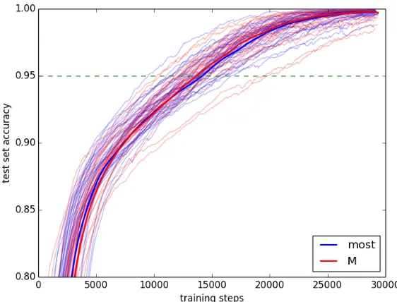
We ran a second experiment, with two quantifiers that are not quite so intimately related. We comparedmost— with the meaning|A∩B|>|A\B|— to an invented non-conservative quantifierM, with the meaning|A|>|B|.46 The learning curves for all 30 trials are plotted in Figure9. Qualitatively, there does not appear to be any significant separation in the learning curves for the two quantifiers. The statistics confirm this appearance. A pairedt-test of the convergence points found that neither quantifier converged significantly earlier than the other (t=0.762,p=0.452).
Figure 9 Experiment 3(b) learning curves. The median at each step is in bold.
These results again pass our sanity check: the model cannot distinguish a con-servative from a non-concon-servative quantifier. The situation is partially analogous to the first experiment: because|A|>|B|is equivalent to|A\B|>|B\A|, the network
early
access
again needs to only learn one pattern, but attach different pairs of labels to it for mostandM. The situation is, however, also partially dis-analogous: because both quantifiers depend onA\Bbut only the latter depends onB\A, the result could have been different. That these two patterned withnot allandnot onlyis then a welcome null result, strengthening the robustness of our sanity check.
In total then, our model at present cannot meet the CHALLENGEwhen it comes
to the CONSERVATIVITYUNIVERSAL. That being said, there are ways of enriching the present setup in ways that may help. In particular, our minimal pair methodology may be a limiting factor. In particular, since neural networks are known to learn to reflect biases in the data that they are trained on,47 it is possible that biasing the data by including more conservative quantifiers than non-conservative ones could make the former easier to learn than the latter. We leave this possibility to future work.
While it thus remains possible that the present model could be enriched so as to make conservative quantifiers easier to learn, we contend that theprima facie
argument at the beginning of this section and our subsequent sanity checks may point to something deeper than a limitation in the current learning model: they could indicate that the source of the CONSERVATIVITY UNIVERSALdiffers from that of the other two universals. In particular, a growing number of researchers argue that conservativity is not a constraint on which quantifiers are lexicalized as determiners but is rather an artifact of the syntax-semantics interface.48 For this reason, many authors develop a so-calledstructuralexplanation of conservativity. While the details of the proposals need not concern us here, the key idea can be explained: while determiners in principle could denote non-conservative quantifiers, the way that the syntax-semantics interface constructs sentence meanings49 renders any sentence with a non-conservative determiner truth-conditionally equivalent to a sentence with a conservative determiner.50 Although nothing in the present paper constitutes an argument for a structural account of conservativity, our null results fit very nicely with such an account: if conservativity ultimately arises as a product of the syntax-semantics interface, it will not be a constraint on the lexicon and so we should not expect its source to be semantic learnability at all.51 This universal
47 See, among others,Bolukbasi et al. 2016,Buolamwini & Gebru 2018. 48 SeeFox 2002,Sportiche 2005,Romoli 2015for accounts of this type. 49 The key ingredient here is the copy theory of movement.
50 Strictly speaking, such sentences might also be trivial. For this reason,Romoli(2015) assumes that trivial meanings are blocked.
early
access
would then fall outside the domain of the CHALLENGE, and so the inability of our model to meet it should not be surprising.52
5 Discussion
In total, our results go a long way in meeting the CHALLENGE: the quantifiers in our experiments that satisfy monotonicity and quantity are easier to learn in our model than those that do not. Moreover, although a conservative quantifier is not easier to learn than a non-conservative one, we argued that there are independent reasons to expect the source of that universal to be different than the first two. In this discussion section, we clarify the nature of our argument by discussing three possible objections: that we study non-lexicalized quantifiers, that a notion of semantic complexity really drives the results, and that our learning model is unrealistic.
First, one may feel uneasy that in some of our experiments, the quantifier satisfy-ing the proposed universal appears not to be lexicalized in any language. This holds fornot allandat most 3.53 First, we note that even though no specific quantifierat most nis lexicalized, cardinalfewis contextually equivalent to some such quantifier. More importantly, however, our argument only delineates the class of quantifiers that are candidates for lexicalization. That is to say, we intend to put upper bounds on what quantifiers simple determiners can denote, but not to exactly demarcate the set of quantifiers denoted in every language. Because exactly which quantifiers satis-fying a given universal are denoted by simple determiners varies across language,54 our goal has been to show merely that quantifiers satisfying the universal are easier to learn and so are better targets for lexicalization.
Second, one might argue that what really explains the universals is a notion of ‘semantic complexity’, together with the thesis that simple expressions tend to denote less complex meanings. At an intuitive level, this seems to make the same predictions as our results.at least 6 or at most 2, being a disjunction of an upward and a downward monotone quantifier, is more complex than bothat least 4andat most 3. Similarly,first 3, which requires checking that noA\Bis observed before threeA∩Bare, can be argued to be more complex thanat least 3, which only needs to look atA∩B. And, as discussed in the preceding section,not allandnot onlyappear
52 We note that it remains unsolved how to account for ‘only’ and reverse-proportional ‘many’ on this structural account of conservativity. Perhaps this provides more reason for arguing that those are not in fact determiners. See footnote21.
53 If one thinks bare numerals only have an ‘exactly’ interpretation, thenat least 4would also not be lexicalized. Because, however, it’s common to have bare numerals denoteat least nand to derive the
exactly ninterpretation pragmatically, we consider it a candidate to be lexicalized.
early
access
to be of equal complexity. Perhaps, then, complexity is the fundamental notion that explains the universals, either by itself explaining learnability or independently.
We present two responses to this line of thought, both hinging on the importance of moving beyond an intuitive notion of semantic complexity to a precise and robust one. On the one hand, because no such notion has been developed and finding one will be difficult, one can view learnability by a recurrent neural network as a kind of operationalization of semantic complexity. That is to say: the best notion of complexity that we have on hand right now just is our notion of learnability. So until an independent and robust general definition of semantic complexity appears, it will be hard to tease apart whether complexity or learnability is more fundamental in the explanation of semantic universals.
On the other hand, there will be difficulties in developing such a notion. First, while the application of tools from computational complexity theory to the semantics of quantifiers have motivated plausible cognitive models,55 these tools do not make sufficiently fine-grained distinctions to explain the universals we are interested in. So consider, again, the intuitive explanation for why our monotone quantifiers are simpler than the non-monotone ones: the latter aredisjunctive, while the former are not. And certainly disjunctive quantifiers will be more complex than non-disjunctive ones. This suggests that something like description length in a mental representation language captures semantic complexity.56 But, as has been known for a long time, what counts as simple according to measures like this depends on what the primitives are.57 As an example, consider the non-monotone quantifier exactly n. This is equivalent toat least n and at most n, and so could be argued to be more complex. But that’s only if the latter two quantifiers are more primitive. After all,at least n is equivalent toexactly n or more than n. None of these considerations entail that no notion of semantic complexity can be given; rather, they point to difficulties that will need to be overcome if the intuition is to be made precise. We would welcome a proposal that does overcome these difficulties.
Finally, one can worry that our model of learning does not resemble the sort of learning that children do when learning the meanings of expressions in natural language. The most fundamental worry here concerns the fact that children tend to learn from positive examples, whereas our model requires an even balance of
55 See, e.g.,McMillan et al. 2005,Szymanik & Zajenkowski 2010.Szymanik(2016) presents and discusses much of this work.
56 SeeTenenbaum et al. 2011for an overview.Piantadosi(2013) applies the framework to quantifier learning, though with different motivations.Kemp & Regier (2012) uses description length in grammars to explain universal properties of kinship systems in language.Feldman(2000) shows that Boolean complexity of binary feature concepts correlates with their ease of learning.
57 See, for instance, the New Riddle of Induction inGoodman 1955, where it is noted that ‘green’ and ‘blue’ become definable if ‘grue’ and ‘bleen’ are taken as primitives. The paperPiantadosi et al. 2016
early
access
positive and negative examples.58 It is true that,ceteris paribus, one would like a model of learning as close to what is known about the acquisition of quantifiers as possible. Minimally, however, the work presented here stands as a proof of concept: our CHALLENGEwas to provideamodel of learning on which quantifiers satisfying universals are easier to learn than those that do not. We have succeeded on that front and, to that end, demonstrated that the CHALLENGEis not in principle unsolvable. Furthermore, while the exact details of our model may diverge from the best models of acquisition, we do find it plausible that there will be ‘cross-model’ transfer: the features that make, for instance, monotone quantifiers easier to learn for our model than non-monotone quantifiers are likely to make them easier to learn for other models as well.
6 Conclusion
Let us take stock. In this paper, we have been developing a particular kind of answer to the question about the origin of semantic universals. According to this answer, such universals arise because expressions satisfying the universal are easier to learn than those that do not. This results in a CHALLENGE: develop a model of learning
on which the former claim holds. In this paper, we have done just that. In particular, we have shown how to train a long short-term memory neural network to learn to verify quantified sentences and explored three semantic universals for quantifiers: monotonicity, quantity, and conservativity. For the first two universals, our model adeptly meets the challenge: monotone and quantitative quantifiers are learned faster than those that do not. This does not hold true for conservativity; but there are independently motivated arguments to suggest that conservativity has a different source than the other universals.
While these results constitute a promising answer to the CHALLENGE, future
work can extend in several different directions. Firstly, we can conduct more and larger experiments. For example, instead of our minimal pair methodology, one would like to train asinglenetwork to learn a significantly wider range of quantifiers, using the semantic properties of the quantifiers as predictors for the rate of learning. Technical limitations prevent this approach currently. Secondly, one would like to develop tools to ‘look inside’ the black box of our trained networks and see how they actually operate. For example, is there a sense in which they learn to verify quantifiers in a way analogous to semantic automata,59 which are computational devices for verifying quantifiers? Thirdly, similar experiments could be run for other semantic
58 Note that here a positive example is not explicitly a grammatical sentence, but a pairing of a sentence with a scenario in which it is true.
early
access
universals, both within the quantifier domain and in other linguistic domains.60 As an example,convexityof denotations for nouns and adjectives seems robust and mirrors monotonicity for quantifiers.61 More concretely, see Steinert-Threlkeld 2018for a similar approach to explaining a semantic universal about responsive verbs. Finally, recall that the general structure of our learnability argument depends on a linking hypothesis: expressions that are easier to learn are more likely to be lexicalized. One would like to embed our neural networks inside of explicit models of language evolution to also corroborate this hypothesis. We hope to pursue all of these avenues in future research.
References
Abadi, Martín, Paul Barham, Jianmin Chen, Zhifeng Chen, Andy Davis, Jeffrey Dean, Matthieu Devin, Sanjay Ghemawat, Geoffrey Irving, Michael Isard, Man-junath Kudlur, Josh Levenberg, Rajat Monga, Sherry Moore, Derek G Murray, Benoit Steiner, Paul Tucker, Vijay Vasudevan, Pete Warden, Martin Wicke, Yuan Yu & Xiaoqiang Zheng. 2016. TensorFlow: A System for Large-Scale Machine Learning. In12th USENIX Symposium on Operating Systems Design and Implementation (OSDI ’16), 265–284. https://www.usenix.org/system/files/ conference/osdi16/osdi16-abadi.pdf.
Bach, Elke, Eloise Jelinek, Angelika Kratzer & Barbara H Partee (eds.). 1995. Quan-tification in Natural Languages, vol. 54 Studies in Linguistics and Philosophy. Springer. https://doi.org/10.1007/978-94-017-2817-1.
Barwise, Jon & Robin Cooper. 1981. Generalized Quantifiers and Natural Language.
Linguistics and Philosophy4(2). 159–219. https://doi.org/10.1007/BF00350139. Bengio, Yoshua. 1991. Artificial Neural Networks and their Application to Sequence
Recognition. Montreal: McGill University dissertation. http://digitool.library. mcgill.ca/R/-?func=dbin-jump-full&object_id=70220.
van Benthem, Johan. 1984. Questions About Quantifiers. The Journal of Symbolic Logic49(2). 443–466. https://doi.org/10.2307/2274176.
van Benthem, Johan. 1986. Essays in Logical Semantics. Dordrecht: D. Reidel Publishing Company. https://doi.org/10.1007/978-94-009-4540-1.
60 Another natural candidate is EXTENSIONALITY, which says that the carrier set of the model is in some ways irrelevant: ifA,B⊆M⊆M0, thenhM,A,Bi ∈Qif and only ifhM0,A,Bi ∈Q. We find it plausible that this universal will pattern with CONSERVATIVITYin not being explainable by our model, but note that the two go hand-in-hand: a typeh1,1iquantifier satisfies both universals exactly when it is therelativizationof a typeh1iquantifier (Peters & Westerståhl 2006, pp. 141-143). This fully captures the asymmetric role played by the restrictor of a determiner.
early
access
Bolukbasi, Tolga, Kai-Wei Chang, James Zou, Venkatesh Saligrama & Adam Kalai. 2016. Man is to Computer Programmer as Woman is to Homemaker? Debiasing Word Embeddings. In Advances in Neural Information Processing Systems (NIPS 29), https://papers.nips.cc/paper/6228-man-is-to-computer-programmer-as-woman-is-to-homemaker-debiasing-word-embeddings.pdf.
Buolamwini, Joy & Timnit Gebru. 2018. Gender Shades: Intersectional Accuracy Disparities in Commercial Gender Classification. InConference on Fairness, Accountability and Transparency, in Proceedings of Machine Learning Research, vol. 81, 77–91. http://proceedings.mlr.press/v81/buolamwini18a/buolamwini18a. pdf.
Chemla, Emmanuel, Brian Buccola & Isabelle Dautriche. 2018. Connecting content and logical words. Accepted atJournal of Semantics. https://semanticsarchive. net/Archive/WVhYzUwM/Chemla-Buccola-Dautriche-ConnectWords.pdf. Chomsky, Noam. 1965. Aspects of the Theory of Syntax. Cambridge: The MIT
Press.
Chomsky, Noam. 1980. Rules and Representations. Oxford: Basil Blackwell. Croft, William. 1990. Typology and Universals. Cambridge: Cambridge University
Press.
Dixon, R.M.W. 1977. Where have all the adjectives gone? Studies in Language
1(1). 19–80. https://doi.org/10.1075/sl.l.l.04dix.
Donahue, Jeff, Lisa Anne Hendricks, Marcus Rohrbach, Subhashini Venugopalan, Sergio Guadarrama, Kate Saenko & Trevor Darrell. 2017. Long-Term Recur-rent Convolutional Networks for Visual Recognition and Description. IEEE Transactions on Pattern Analysis and Machine Intelligence 39(4). 677–691. https://doi.org/10.1109/TPAMI.2016.2599174.
Elman, Jeffrey L. 1990. Finding Structure in Time. Cognitive Science 14(2). 179–211. https://doi.org/10.1207/s15516709cog1402_1.
Feldman, Jacob. 2000. Minimization of Boolean Complexity in Human Concept Learning. Nature 407(05 October 2000). 630–633. https://doi.org/10.1038/ 35036586.
von Fintel, Kai. 1997. Bare Plurals, Bare Conditionals, and Only. Journal of Semantics14(1). 1–56. https://doi.org/10.1093/jos/14.1.1.
von Fintel, Kai & Edward L Keenan. 2018. Determiners, Conservativity, Witnesses.
Journal of Semantics35(1). 207–217. https://doi.org/10.1093/jos/ffx018. von Fintel, Kai & Lisa Matthewson. 2008. Universals in semantics. The Linguistic
Review25. 139–201. https://doi.org/10.1515/TLIR.2008.004.
Fox, Danny. 2002. Antecedent-Contained Deletion and the Copy Theory of Movement. Linguistic Inquiry 33(1). 63–96. https://doi.org/10.1162/ 002438902317382189.
early
access
Gierasimczuk, Nina. 2007. The Problem of Lerning the Semantics of Quantifiers. In Balder ten Cate & Henk Zeevat (eds.),6th International Tbilsi Symposium on Logic, Language, and Computation (TbiLLC), vol. 4363 Lecture Notes in Computer Science, 117–126. https://doi.org/10.1007/978-3-540-75144-1_9. Gierasimczuk, Nina. 2009. Identification through Inductive Verification:
Appli-cation to Monotone Quantifiers. In P Bosch, D Gabelaia & J Lang (eds.),
7th International Tbilsi Symposium on Logic, Language, and Computation (TbiLLC), vol. 5422 Lecture Notes in Artificial Intelligence, 193–205. https: //doi.org/10.1007/978-3-642-00665-4_16.
Gisiger, Thomas & Mounir Boukadoum. 2011. Mechanisms gating the flow of information in the cortex: what they might look like and what their uses may be.
Frontiers in Computational Neuroscience5(1). 1–15. https://doi.org/10.3389/ fncom.2011.00001.
Goodfellow, Ian, Yoshua Bengio & Aaron Courville. 2016. Deep Learning. The MIT Press. https://www.deeplearningbook.org/.
Goodman, Nelson. 1955. Fact, Fiction, & Forecast. Cambridge, MA: Harvard University Press.
Graves, Alex. 2013. Generating Sequences With Recurrent Neural Networks. https: //arxiv.org/abs/1308.0850.
Hackl, Martin. 2009. On the grammar and processing of proportional quantifiers:
mostversusmore than half. Natural Language Semantics17(1). 63–98. https: //doi.org/10.1007/s11050-008-9039-x.
He, Haibo & Edwardo A. Garcia. 2009. Learning from Imbalanced Data. IEEE Transactions on Knowledge and Data Engineering 21(9). 1263–1284. https: //doi.org/10.1109/TKDE.2008.239.
Hengeveld, Kees, Jan Rijkhoff & Anna Siewierska. 2004. Parts-of-speech systems and word order. Journal of Linguistics40(3). 527–570. https://doi.org/10.1017/ S0022226704002762.
Hochreiter, Sepp & Jürgen Schmidhuber. 1997. Long Short-Term Memory. Neural Computation9(8). 1735–1780. https://doi.org/10.1162/neco.1997.9.8.1735. Hunter, Tim & Jeffrey Lidz. 2013. Conservativity and learnability of determiners.
Journal of Semantics30(3). 315–334. https://doi.org/10.1093/jos/ffs014. Hyman, Larry M. 2008. Universals in phonology. The Linguistic Review25(1-2).
83–137. https://doi.org/10.1515/TLIR.2008.003.
Jordan, Michael I. 1986. Serial Order: a Parallel Distributed Processing Approach. Tech. Rep. ICS-8604. https://pdfs.semanticscholar.org/f8d7/ 7bb8da085ec419866e0f87e4efc2577b6141.pdf.
early
access
Katsos, Napoleon, Chris Cummins, Maria-José Ezeizabarrena, Anna Gavarró, Jelena Kuvaˇc Kraljevi´c, Gordana Hrzica, Kleanthes K. Grohmann, Athina Skordi, Kristine Jensen de López, Lone Sundahl, Angeliek van Hout, Bart Hollebrandse, Jessica Overweg, Myrthe Faber, Margreet van Koert, Nafsika Smith, Maigi Vija, Sirli Zupping, Sari Kunnari, Tiffany Morisseau, Manana Rusieshvili, Kazuko Yatsushiro, Anja Fengler, Spyridoula Varlokosta, Katerina Konstantzou, Shira Farby, Maria Teresa Guasti, Mirta Vernice, Reiko Okabe, Miwa Isobe, Peter Crosthwaite, Yoonjee Hong, Ingrida Balˇciunien˙e, Yanti Marina Ahmad Nizar, Helen Grech, Daniela Gatt, Win Nee Cheong, Arve Asbjørnsen, Janne von Koss Torkildsen, Ewa Haman, Aneta Mi ekisz, Natalia Gagarina, Julia Puzanova, Darinka An ¯delkovié, Maja Savi´c, Smiljana Joši´c, Daniela Slanˇcová, Svetlana Kapalková, Tania Barberán, Duygu Özge, Saima Hassan, Cecilia Yuet Hung Chan, Tomoya Okubo, Heather van der Lely, Uli Sauerland & Ira Noveck. 2016. Cross-linguistic patterns in the acquisition of quantifiers. Proceedings of the National Academy of Sciences 113(33). 9244–9249. https://doi.org/10.1073/ pnas.1601341113.
Keenan, Edward L. & Denis Paperno (eds.). 2012. Handbook of Quantifiers in Natural Language, vol. 90 Studies in Linguistics and Philosophy. Dordrecht: Springer Netherlands. https://doi.org/10.1007/978-94-007-2681-9.
Keenan, Edward L & Jonathan Stavi. 1986. A Semantic Characterization of Natural Language Determiners. Linguistics and Philosophy 9(3). 253–326. https: //doi.org/10.1007/BF00630273.
Keenan, Edward L & Dag Westerståhl. 1997. Generalized Quantifiers in Linguistics and Logic. In Johan van Benthem & Alice ter Meulen (eds.),Handbook of Logic and Language, 837–893. Elsevier. https://doi.org/10.1016/B978-044481714-3/50020-5.
Kemp, Charles & Terry Regier. 2012. Kinship categories across languages reflect general communicative principles. Science336(6084). 1049–1054. https://doi. org/10.1126/science.1218811.
Kingma, Diederik P. & Jimmy Ba. 2015. Adam: A Method for Stochastic Op-timization. InInternational Conference of Learning Representations (ICLR), https://arxiv.org/abs/1412.6980.
Kotek, Hadas, Edwin Howard, Yasutada Sudo & Martin Hackl. 2011a. Three Readings of Most. In Neil Ashton, Anca Chereches & David Lutz (eds.),
Semantics and Linguistic Theory (SALT 21), 353–372. https://doi.org/10.3765/ salt.v0i0.2621.
early
access
Lindström, Per. 1966. First order predicate logic with generalized quantifiers.
Theoria32(3). 186–195. https://doi.org/10.1111/j.1755-2567.1966.tb00600.x. May, Robert. 1991. Syntax, Semantics, and Logical Form. In Asa Kasher (ed.),The
Chomskyan Turn, Blackwell Publishers.
McMillan, Corey T, Robin Clark, Peachie Moore, Christian Devita & Murray Gross-man. 2005. Neural basis for generalized quantifier comprehension. Neuropsy-chologia43(12). 1729–1737. https://doi.org/10.1016/j.neuropsychologia.2005. 02.012.
McNab, Fion