Issues
ISSN: 2146-4138
available at http: www.econjournals.com
International Journal of Economics and Financial Issues, 2018, 8(4), 206-213.
Exchange Rate and Turkish Tourism Trade
Ferhat Citak*
Hitit Üniversitesi İİBF Bankacılık ve Finans Bölümü, Corum, Turkey. *Email: ferhatcitak@hitit.edu.tr
ABSTRACT
The aim of this paper is to analyze the relationship between the exchange rate and tourism trade in Turkey from 1970 to 2016 by applying three vector autoregression models. The main findings of this paper can be documented as follows: (1) There is no long-run cointegration relationship among the variables (2) the reaction of the export revenue to an unexpected 1% depreciation exchange rate shock is positive and statistically significant at the 95% level (3) import tourism spending exhibits a robust significant positive response to home demand shock (4) the response of trade balance to 1% shock in the exchange rate is negative and significant, which shows the evidence of J-curve behavior for the selected eight European countries.
Keywords: Trade Balance, Turkish Tourism,J-Curve, Cointegration, Vector Autoregression
JEL Classification: E21
1. INTRODUCTION
In today’s world, tourism is akin to globalization. Tourism, in this regard, is the movement of peoples from one part of the world to another. But in this instance, this is a temporary stage and these people usually come back to the place where they started their travel. This pursuit is usually to become aware of different cultures, dance, music, clothes, and languages of other places of interest.
With the world becoming what is termed a “global village,” tourism too is getting enhanced in some ways. It could be business tourism, where one goes to another place with regard to one’s occupation for professional reasons. One could be going for religious tourism purposes, where a traveler is in search of enhancement of knowledge of a given religion or is on a pilgrimage. Tourism could also be just for satisfying an inner desire to travel to unknown or exotic destinations or for the thrill of the adventure involved in some activity. Whatever the case, tourism has a direct effect bearing on globalization since the more we travel, the more global in our outlook and thinking we become.
International tourist arrivals increased by about 4.4% in the year 2015 (WTO, 2016). About 50 million additional tourists, by this we mean overnight visitors, went to international places in comparison with the year before (WTO, 2016). Also, international tourist
arrivals to the European Union (EU) increased by 4% in the year 2016. Translating into terms of world tourism, this is about 40% of entire travel (UNWTO, 2017). As far as Turkey is concerned, the number of foreigners in Turkey came down by 3.96% in March 2017 from 1.65 million in the same month previous year (Trading Economics, 2017).
Tourism has several positive impacts. First and foremost, it is a source of employment creation. Also, it goes a long way in enhancing a country’s image on a global platform. It helps not just to preserve the traditions, customs and culture of any given place, but also spreads them to the home countries of the tourists. In addition, it brings foreign exchange to the country, thereby helping the economy.
Moreover, tourism may help to improve a locale place – with visitors coming in there may be improvements in cleanliness, environment enhancement and other benefits. Local industry
and handicrafts boost since visitors tend to purchase items for
memorabilia and gifting purposes. However, some of the negative
aspects associated with tourism are that it puts pressure on the
The remainder of this paper is structured as follows. The first section overviews the profile of the Turkish tourism market. The next section summarizes the relevant literature and highlights the main contributions of this research. The following sections briefly describe the model, methodology, the data, and report the empirical findings. Finally, the last section reports the main conclusions of the study.
2. A PROFILE OF TURKISH TOURISM
MARKET
Tourism is an important element of international trade and one of the largest investment and development industries affecting local, regional, national and global economies in the world (Akay et al., 2017). It offers a large amount of economic benefits such as generating new job opportunities, encouraging the private sector, helping to improve per capita income and standard of living, facilitating development of basic infrastructural facilities, creating a multiplier impact on a national economy, and reducing poverty (Saayman and Saayman, 2015). It is a noteworthy point that tourism as a field needs a lesser scale of per capita funds. Even the technological as well as labor related skills necessary for this sector are on the lower side. Also, tourism encounters much less of a protectionist attitude in world economies than manufacturing does. Thus, tourism has become an appealing arena to explore for lesser developed places and countries looking for methods for economic development (Sharma, 2004).
Thanks to its great geographical location and natural opportunities, and its many historical, religious, and archaeological sites, Turkey is one of the leading countries in tourism. Since free market economy policies and government’s promotion of tourism in the 1980s, tourism has come to play a major role in the Turkish economy. The Tourism Encouragement Law of 1982 put tourism among the “sectors of special important for development.” In addition, the Turkish government introduces many incentives – such as exceptions from several taxes including customs and export taxes, the transfer of public land to private tourism companies, low interest loans to the investors through the Turkish Tourism Bank, investment allowance, concessional tariff rates for power, water, and gas consumption - to boost the tourism sector (Özen and Kuru, 1998; Nohutcu, 2002; Yolal, 2016). As a result of these incentive policies, tourism experienced a remarkable success after the mid-1980s.
For the reasons stated above, the number of international visitors coming to Turkey increased almost thirty-five times, rising from 725 thousand in 1970 to 39.4 million in 2015. According to World Tourism Organization report, in 2016 Turkey held 6th place in the
international ranking of the “Top 10” tourist destination assessed by the number of arrivals. In addition, in terms of tourist revenue, in 2016 Turkey occupied 12th place in the international tourist
receipts. According to the World Tourism Org.UNWTO. (2017, tourism contributes 12.5% to Turkish gross domestic product (GDP).
It is also important to note that the Turkish tourism industry, in 2016, faced difficulties such as the downing a Russian warplane
by a Turkish jet in November 2015, the terrorist attack on Istanbul’s Ataturk airport in June 2016, and a failed military coup attempt in July 2016. The number of tourist arrivals to Turkey amounted to 25 million, a decrease by 41% compared to 2015. In addition, according to data compiled the Republic of Turkey Ministry of Culture and Tourism, during the first quarter of 2017, Turkey welcomed 3.8 million tourists, a 6.43% decrease over the corresponding period of 2015.
During 2007-2016, about 50% of inbound tourists staying in Turkey came from the EU countries (Turk Stat, 2017). The top twelve tourists’ origin countries are, on average, Germany, Russia, the United Kingdom, Bulgaria, Iran, Georgia, the Netherlands, France, USA, Ukraine, Greece, and Italy. Furthermore, the number of visitors from Germany, Russia, the Netherlands, France, USA, Italy and Greece has significantly declined in recent times.
3. REVIEW OF RELATED LITERATURE
There is an old saying, “the world is a great book, of which they that never stir from home read only a page” (St. Augustine, 354-430, AD). Indeed, travelling the world enables one to see a lot of things and gain experience concerning different cultures. Failing to travel would make one remain within his or her cultural setting. Therefore, one would not be updated on many issues.
There is a multitude of previous studies on tourism. For example, Vogt (2008) analyzes the real income and relative elasticity of demand in tourism exports and imports. The study makes use of data from the year 1973 to 2002. The findings show that the response of the trading partners to the changes in real income in tourism may have an impact on tourism in the country by increasing surpluses on the tourism balance of trade in the country. The spending of people from these countries in the United State enables trade in tourism to improve as they bring in foreign exchange. The rates of exchange partly determine the choice of foreign tourists coming to the country.
In their research note, Thompson and Thomson (2010) discuss the effects of exchange rates and the adoption of the euro in tourism revenue in Greece using a sample period of 32 years. The paper identifies that tourism is a crucial factor in the economy of the country. It earns the country a lot of foreign exchange. The results of the study show that the rates of exchange have an impact on tourism in Greece. A depreciation of the rates of exchange enables the country to earn more foreign exchange in tourism. It also shows
that the adoption of the euro had a positive impact on tourism in
Greece. It makes the country at par with other European countries since they have the same currency.
travelling outside the country for tourism is considered a luxury. However, it is common for people to travel to the United States
for tourism.
Cheng et al. (2013b) discuss the effects of real exchange rates and income on tourism in the United States. The paper analyzes the revenue earned by exporting tourism and spending on imports using the data available between the years of 1973-2010. The results of the study show that depreciation has a positive impact on the revenue earned from tourism exports. However, it does not affect import spending on tourism in the country. The paper also states that when the exchange rates drop, tourists have more to spend, increasing foreign income from tourism. However, local tourists have no impact since they spend local currency.
More recently, Chi (2015) examines the effects of income and exchange rates on the exports and imports of tourism in the country. He explained the trends with an aim to help understand
the determinants of the balance of trade in the tourism sector in
the United States. The findings of the study show that appreciation of the dollar has a negative impact on the trade balance in tourism in the country. The paper also notes that the appreciation of the dollar makes the exchange rates unfavorable for tourists, thereby making them avoid the country as a tourist destination.
Turning to the domestic literature, a few empirical studies have been carried out on tourism development for Turkey. For instance, Halicioglu (2010) analyzes the demand for tourism in Turkey with regard to international exchange rates and income. The results show that depreciation in international exchange rates has a positive impact on the demand for tourism, thereby leading to a positive trade balance in tourism. Favorable exchange rates enable the tourists to spend more local currency in the country.
Kiliç and Bayar (2014) discuss the relationship between the volatility of the exchange rates and expenditure on tourism in Turkey using annual data from 1994 to 2013. The Johansen co-integration test is used to get the relationship between the series. The results of the study show that there is a positive relationship between the rates of exchange in the country and expenditures on tourism. When the exchange rates depreciate, international tourists are attracted to the country leading to an increase in foreign income, which helps improve the tourism sector. In addition, Akay et al. (2017) analyzed the effects of income and exchange rates on tourism in Turkey by applying Johansen’s maximum likelihood approach to measure the long-term impact of the exchange rates and income on tourism in the country. They report that income is the most important factor that can explain the trade balance in tourism over the long-term. In particular, the results show that foreign income and real exchange rates affect tourism in a positive manner, while domestic income affects tourism in a negative manner. Furthermore, they point out that when the rates of exchange are low, foreign income for the tourists would increase, making more people choose the destination, but domestic income has no effect on tourism since there is no foreign exchange involved.
This paper extends the Turkish tourism literature in two ways. First, this study focuses on the dynamic interactions among the
variables by applying a multivariate vector autoregression (VAR) framework, which does not provide the short-run and long-run effects of the exchange rates on tourism. Second, using annual data for the period 1970-2016, this study analyzes the presence of J-curve for the eight major Turkey tourist arrival EU countries: Austria, Belgium, France, Germany, Greece, Netherlands, Italy, and Portugal.
4. THEORETICAL FRAMEWORK FOR
TOURISM TRADE
In dealing with the tourism trade balance analysis, this paper follows similar equation chosen from Vogt (2008), Cheng et al. (2013a; 2013b), and Chi (2015), which examines the relationship between exchange rate and tourism trade balance. The linear models for Turkish exports (Xt) and imports (Mt) of tourism are specified as below:
EXt f Yt Et= ( *, ) (1)
IMt =f (Yt,Et) (2)
where is the export revenue, Mt is the import spending, Yt is
Turkey’s income,is foreign income, and Et is the exchange rate of Turkish lira against foreign currencies. Equation (1) and (2) are rewritten in a double-log functional form, and we have.
ln Xt = a0+a1lnY*+a2lnEt+εt (3)
lnMt = b0+b1lnY+b2lnEt+ϑt (4)
In the literature, trade balance is usually measured as the difference between export revenue and import spending. In this study, following a similar approach proposed by Bahmani-Oskoosee and Brooks (1999), Boyd et al. (2001), Onafowora (2003) and Cheng et al. (2013a; 2013b), we measure the trade balance as the ratio of export revenue and import spending, B ≡ X/M. After taking natural logarithm, we specify trade balance equation as follows:
lnBt = ln Xt−ln Mt (5)
Substituting Equations (3) and (4) into (5), we get:
lnBt=(a0–b0)+a1 lnY*–b1 lnY+(a2–b2) lnEt+(εt–ϑt) (6)
To understand the correlation between the tourism trade and exchange rate, one must consider the J-Curve phenomenon. J Curve serves as an example of movement in variables that declines in the beginning and then gradually increases to the new higher levels than the starting point forming the shape of letter “J” on time series graph.
due to higher costs of imports and lesser. With the passage of time, the situation of exports improves due to devaluation in the country, thereby, giving competitive advantage to the country to trade in the world and also, imports start declining due to the availability of cheaper products at the domestic market compared with the imported goods. This situation brings in positive effects in the balance of payments and the net balance of payments becomes positive giving a “J” curve effect in the economy (Staff, 2003).
5. DATA AND EMPIRICAL METHODOLOGY
5.1. DataAs noted in the introduction, in this study, tourist arrivals from eight member countries of EU: Austria, Belgium, France, Germany, Greece, Italy, Netherlands, and Portugal are considered. These countries have been selected on the basis of tourism demand for Turkey from EU. To avoid the seasonality problem, data consists of annual observations during the period 1970 -2016. Secondary data sources were used in the study and are collected from various sources. Data for tourism arrivals for the period 1970-2016 are obtained from Turkish Statistical Institute (TURKSTAT). Turkey’s income is GDP and we record income for the rest of the world as the sum of GDP of the selected countries. The foreign exchange is measured as the price of a dollar in terms of Turkish liras. All GDPs are obtained from the World Bank. All variables are expressed in natural log form.
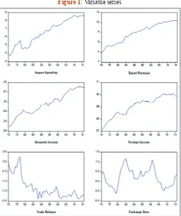
Figure 1 presents the plots of all variables in natural logs. Tourism export revenue, X, generally shows an increasing trend since 1970, while there are some fluctuations in import spending, M, between
the years. In addition, trade balance, B, is always negative except mid- 1970s. The exchange rate, E, had three periods of Turkish lira depreciation, up to late 1970s then during the mid-1990s, and again up to 2007s, then two periods of appreciation, from 1982 to 1985 and from 1998 to 2001. Over the period 1970-2016, Turkey’s income,, and foreign income,, fluctuates between the years.
5.2. Empirical Methodology
This study applies the method of time series econometrics, which is VAR estimation technique to model the exchange rate and tourism trade balance in Turkey. The VAR model is a multi-equation system in which all variables are treated as endogenous and jointly determined. The VAR model helps to investigate the
interrelations between the variables and each dependent variable
are regressed against their own and each other’s lagged values in the system (Enders, 2004).
As stated previously, we use three VAR econometric models. First, the export model is based on a tri-variate VAR (p) with the exchange rate rt, tourism export xt, and foreign income . Second, the import model is based on a tri-variate VAR (p) with the exchange rate rt, tourism import mt and home income yt. Third, the tourism balance model is a quad-variate VAR (p) with the exchange rate rt, tourism balance bt = xt–mt, foreign income, and
home income yt. The relationship between the three time series:
xt, mt, and bt takes the following form:
xt =a1+∑pj=1b1j xt j +− ∑qj=1β2j rt j +− ∑rj=1β3j yt j* + 1t− ε ,
(Model 1)
mt=α1+∑pj=1y1j mt j− +∑qj=1y j rt j2 − +∑rj=1y3j yt j 2t− +ε ,
(Model 2)
bt pj 1j bt j qj j rt j
3j yt j j
r
j rt j j
q
= +∑ = − +∑ = − +
− =
∑ + = − +
α θ θ
θ θ
1 1 1 2
1 * ∑∑ 1 4 ε3t
(Model 3)
Where, xt mt, and bt, are dependent variables, α1,α2, and α3 are the intercepts xt–j, mt–j, and bt–j are the lagged values of interested variables, and εit are error terms that are assumed to be normally
distributed and white noise.
Building a VAR model involves several stages. First, time series variables should be tested for unit roots individually to determine their respective orders of integration by using common unit root tests, such as Augmented Dickey-Fuller (ADF) or Philips-Perron (PP). Second, the appropriate lag length of the VAR should be determined through the use of optimum lag length selection criteria, such as the Akaike Information Criterion (AIC) or the Schwarz Bayesian Criterion (SBC). Third, the Johansen’s (1998) co-integration test should be applied to analyze the long-term relationship among the variables. Lastly, the Impulse Reaction Function (IRF), which refers to the reaction of any dynamic system to an external shock, and variance decomposition analysis, can be used to examine the inter-relationship among
the variables. Figure 1: Variable series
6. RESULTS OF DATA ANALYSIS
6.1. Descriptive StatisticsThe descriptive statistics of data is reported in Table 1. This paper uses yearly data covering from 1970 to 2016 with 47 observations for each variable. The exchange rate has a smaller standard deviation among all the variables. The maximum growth rate of exchange rate was 1.33%, whereas the minimum was −0.09%. On the other hand, the minimum trade balance over the entire period was −1.88% as against the maximum of 0.27%.
6.2. Stationary Pre-test Results
Time series data often non-stationary and this situation could cause the problem or spurious regression and biased results (Maddala, 2001). In this study, the Augmented-Dickey-Fuller (ADF) and Philips-Perron (PP) tests, the null hypothesis is non- stationary, are applied to determine the stationary of all variables. Table 2 reports the results of unit root in each variable. Both unit root tests are in agreement that all the variables are non-stationary in
levels but their first differences are stationary at the 1% level. In other words, the results confirm that all the variables are integrated process of first order, I(1).
6.3. Co-integrating Analysis and VAR Model Checking
Before proceeding to Johansen’s co-integration analysis, optimal lag length (p) is determined using a VAR model. The choice of the optimum number of lags was made using Akaike (1974; 1976), Schwarz (1978), and Hannan-Quinn (1979) criteria. Table 3 shows the results of VAR lag order selection criteria for three tests. The maximum possible lag length considered in each model is 4 (years). For Model 1, all three criteria select an optimal lag length of one; therefore we select VAR (1). For Model 2, the SIC and HQC criteria select a VAR (1) model while the AIC criteria selects a VAR (2). But, as the lag one has serial correlation problem, we select VAR (2) for model 2. Finally, for Model 3, all three criteria suggest the lag one; thus we choose VAR (1) for model 3. Once the optimal lag length is chosen, the next step is to determine the existence of long-run relationship between variables. To test for co-integration, the Johansen’s (1998) co-integration test is applied to detect the long-term relationship between the variables. Engle and Granger (1987. p. 264) states that, “it may not be easy to test whether a set of variables are co-integrated before estimating a multivariate dynamic model.” Table 4 presents the results of the Johansen multivariate co-integration test for all three systems of equations. As seen from Table 4, two tests, the trace test and maximum eigenvalue test, are employed to test co-integrating among the variables. In Model 1, we examine if there is a long-Table 1: Descriptive statistics
Variable n Mean±SD Max. Min.
Import spending (M) 47 6.589±1.543 8.678 3.742 Export revenue (X) 47 7.904±1.997 10.443 3.943 Home income (Y) 47 25.798±1.171 27.580 23.511 Foreign income (Y^*) 47 29.049±0.847 30.079 27.083 Exchange rate (E) 47 0.570±0.361 1.335 −0.094 Trade balance (B) 47 −1.314±0.570 0.270 −1.888 Source: Turk Stat, (2017). SD: Standard deviation
Table 2: Unit root results of log variables (H0: One unit root; HA: No unit root)
Variables Specification Augmented Dickey-Fuller (ADF) Philip-Perron (PP)
τ τc τc+t τ τc τc+t
Import spending Level 1.38 −1.18 −2.60 1.35 −1.18 −2.73 Differenced −5.75 −6.66 −6.71 −5.81 −6.64 −6.71 Export revenue Level 1.72 −2.25 −1.55 1.42 −2.83 −1.43 Differenced −4.48 −5.96 −6.29 −4.37 −5.91 −6.95 Trade balance Level 0.16 −2.32 −2.73 0.22 −2.31 −2.75 Differenced −7.42 −7.44 −7.42 −7.53 −7.78 −8.25 Exchange rate Level −1.44 −2.69 −2.63 −1.15 −2.23 −2.20 Differenced −4.73 −4.67 −4.64 −4.73 −4.67 −4.69
Home income Level 1.72 −1.45 −2.33 1.71 −1.66 −2.84
Differenced −5.36 −6.77 −6.86 −5.60 −6.78 −6.87 Foreign income Level 2.46 −3.22 −2.25 1.57 −2.96 −1.74 Differenced −3.71 −4.51 −5.03 −3.80 −4.43 −4.94 Test critical values
1% −2.61 −3.58 −4.17 −2.61 −3.58 −4.17
The table reports results of Augmented Dickey-Fuller (ADF) and Philips and Perron (PP) unit root tests. τ, τc and τc+t indicate the model statistics without either constant or trend, with
constant, and with constant and trend, respectively. The number of lags is chosen by the Schwarz Information Criterion (BIC) for the Augmented Dickey-Fuller and the Philips and Perron (PP). Tests for unit roots have been carried out in E views 9.0
Table 3: VAR lag order selection criteria
Lag order Model 1 Model 2 Model 3
AIC SIC HQC AIC SIC HQC AIC SIC HQC
0 3.79 3.91 3.84 4.54 4.66 4.58 3.23 3.39 3.29 1 −3.94* −3.45* −3.76* −2.28 −1.79* −2.10* −5.61* −4.79* −5.53* 2 −3.90 −3.04 −3.58 −2.36* −1.50 −2.04 −5.47 −4.00 −4.93 3 −3.79 −2.57 −3.34 −2.02 −0.79 −1.57 −5.16 −3.03 −4.38 4 −3.89 −2.29 −3.30 −2.08 −0.48 −1.49 −5.21 −2.42 −4.18
run relationship between tourism export revenue, exchange rate, and foreign income, whereas in Model 2, we analyze if tourism import spending, exchange rate, and home income cointegrated in the long-run. In addition, in Model 3, we investigate if there is a long-run relationship between tourism trade balance, exchange rate, home income, and foreign income. According to all maximal eigenvalue and trace statistic tests, all calculated P-values are above the 0.05, thus the results of all three models indicate that we do not reject the null hypothesis that there is no co-integration at the 0.05 level.
6.4. Impulse Response Function
To check the VAR to be stationary, all the inverse roots of the characteristics AR polynomial must lie inside the unit circle. If this is not the case, impulse-response inferences are not valid. In this study, all three VAR models do not have a root outside the unit circle, hence we conclude that all three VAR models are stationary, which allows us to proceed to the impulse response analysis.
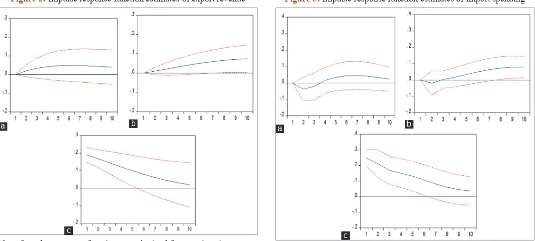
Figure 2: Impulse response function estimates of export revenue
a b
c
Note: Impulse-response functions are obtained from a tri-variate vector autoregression model with the exchange rate ordered first, whereas the foreign demand variable is placed last
Figure 3: Impulse response function estimates of import spending
a b
c
Note: Impulse-response functions are obtained from a tri-variate vector autoregressive model with the exchange rate ordered first, whereas the home demand variable is placed last
Table 4: Results of Johansen’s maximum likelihood tests for multiple co-integrating relationships
Null Hypothesis Model 1 Model 2 Model 3
Test-Stat P-value Test-Stat P-value Test-Stat P-value
Trace test
None (r=0) 35.576 0.0696 29.971 0.0877 58.772 0.0634 At most 1 (r≤1) 15.494 0.1133 14.589 0.0681 28.682 0.0668 At most 2 (r≤2) 3.841 0.1009 4.364 0.0767 7.721 0.4957 Maximum Eigenvalue
None (r=0) 16.406 0.2020 15.381 0.2630 30.089 0.0733 At most 1 (r≤1) 12.690 0.0873 10.224 0.1976 20.961 0.0528 At most 2 (r≤2) 6.480 0.1109 4.364 0.0722 6.949 0.4952
*Indicates the smallest value of the criterion. AIC, Akaike Information Criterion; SIC, Schwarz Information criterion; HQ, Hannan-Quinn Information Criterion. VAR: Vector autoregression
The impulse response functions (IRFs) represent the way a system reacts to the exogenous shocks (Inoue and Kilian, 2013). Estimated export revenue, import spending, and trade balance response functions are reported in Figures 2-4, respectively. Point estimates of the IRFs are plotted with a solid line, whereas the dotted lines
show a two-standard-deviation band around the point estimates.
In the first panel of Figure (2a), export revenue exhibits a robust significant positive response to an unexpected 1% depreciation exchange rate shock that takes 6 years to converge to the steady state. The second panel of Figure (2b) shows a robust nearly elastic positive response to foreign income shocks. Lastly, the third panel of Figure (2c) represents a 1% shock in foreign demand reduces the export revenue at a decreasing rate and converges to equilibrium after 10 years.
period, 85.60% variance in tourism import spending is explained by 3.12% variance in exchange rate and 11.26% of the variance in home income. Similarly, as it is obvious from the Table 7, in the seventh lag period 87.51% variance in tourism trade balance is explained by 8.75% variance in exchange rate, 3.68% variance in home income, and 0.03% variance in foreign income.
7. CONCLUDING REMARKS
The present work explores the dynamic relationship among tourism export revenue, tourism import spending, the exchange rate, the home and foreign income with VARs for yearly data in
Table 5: Export variance decomposition analysis
k s.e. xt rt yt
1 0.189 100.000 0.0000 0.0000 2 0.253 99.222 0.634 0.143 3 0.294 97.613 1.794 0.591 4 0.323 95.327 3.221 1.450 5 0.343 92.497 4.719 2.783 6 0.359 89.264 6.141 4.593 7 0.372 85.781 7.388 6.829 8 0.383 82.200 8.405 9.394 9 0.394 78.661 9.175 12.163 10 0.403 75.278 9.711 15.010 Note: k denotes the forecast horizon in years. Variance decomposition analysis is carried out from a tri-variate VAR model with the export revenue ordered first, whereas the foreign income is placed last. Standard errors (s.e.) are obtained from 5000 nonparametric bootstrap simulations. All results are obtained using E views 9.0
Table 6: Import variance decomposition analysis
k s.e. mt rt yt
1 0.252 100.000 0.0000 0.0000 2 0.336 99.554 0.268 0.176 3 0.389 98.591 0.742 0.666 4 0.426 97.192 1.291 1.516 5 0.454 95.461 1.822 2.716 6 0.475 93.514 2.277 4.208 7 0.493 91.466 2.630 5.902 8 0.508 89.418 2.880 7.701 9 0.521 87.447 3.039 9.512 10 0.534 85.609 3.126 11.263
k denotes the forecast horizon in years. Variance decomposition analysis is carried out from a tri-variate VAR model with the import spending ordered first, whereas the home income is placed last. Standard errors (s.e.) are obtained from 5000 nonparametric bootstrap simulations. All results are obtained using E views 9.0
Table 7: Trade balance variance decomposition analysis
k s.e. bt rt yt
1 0.230 100.000 0.0000 0.0000 0.0000 2 0.257 98.184 1.116 0.680 0.018 3 0.267 95.511 2.872 1.583 0.032 4 0.274 92.915 4.681 2.366 0.036 5 0.279 90.710 6.295 2.957 0.035 6 0.283 88.929 7.652 3.383 0.035 7 0.286 87.515 8.759 3.686 0.038 8 0.288 86.402 9.648 3.902 0.046 9 0.290 85.527 10.353 4.060 0.058 10 0.292 84.841 10.905 4.176 0.076
k denotes the forecast horizon in years. Variance decomposition analysis is carried out from a quad -variate VAR model with an ordering, the trade balance, the exchange rate, the home and foreign income. Standard errors (s.e.) are obtained from 5000 nonparametric bootstrap simulations. All results are obtained using Eviews 9.0. [IJEFI%206659%20ferhatcitak%20okey] IJEFI%206659%20
ferhatcitak%20okey_F4.tif
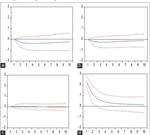
Figure 4: Impulse response function estimates of trade balance.
b
d c
a
Note: Impulse-response functions are obtained from a quad-variate vector autoregression model with ordering of the exchange rate, the home income, the foreign income, and the trade balance
to the steady state after 10 periods. Similarly, Figure (3b) shows that the reaction of import spending to 1% shock in home income shock is negative and not significant at the 90%. In addition, Figure (3c) represents the response of import tourism spending to home demand shock. The results indicate that 1% shock in home demand has a positively significant impact on import tourism spending and decreases over time.
In the trade balance model Figure (4a), the reaction of trade balance to 1% shock in exchange rate is negative and significant at the 95%. It shows as negative in the first two periods and then starts to converge to the steady state. The response of trade balance to foreign income shock is shown in Figure (4b). The results show that an unexpected 1% foreign income shock reduces the trade balance and is significant at the 90%. In addition, Figure (4c) shows how trade balance responds positively to the shocks in home income in the first three periods and as expected, home income lowers the trade balance. But these affects are not significant at any significance level. Lastly, the trade balance represents a robust significant positive response to its own shocks as depicted
in Figure (4d).
6.5. Variance Decomposition Analysis
Turkey over the period of 1970 to 2016. From our estimation results, the export revenue shows a significant positive response to exchange rate shock. However, the response of import tourism spending to home demand shock is positive and statistically significant at the 95% level. Finally, an unexpected 1% exchange rate shock worsens the trade balance initially, and then starts to converge to the steady state. In summary, we conclude that the J-curve hypothesis is only valid for trade balance model for the selected eight European countries.
REFERENCES
Akaike, H. (1974), A new look at the statistical model identification. IEEE Transactions on Automatic Control, AC-19(6):716-23.
Akaike, H. (1976), An information criterion (AIC). Math. Sci., 14 (153):5-9.
Akay, G.H., Cifter, A., Teke, O. (2017), Turkish tourism, exchange rates and income. Tourism Economics, 23(1), 66-77.
Bahmani-Oskooee, M., Brooks, T. J. (1999), Bilateral J-curve between US and Her Trading Partners. Weltwirtschaftliches Archives, 135(1): 156-165.
Boyd D, Caporale, G.M., Smith, R. (2001), Real Exchange Rate Effects on the Balance of Trade: Cointegration and the Marshall-Lerner Condition. International Journal of Finance and Economics, 6, 187-200.
Cheng, K.M., Kim, H., Thompson, H. (2013a), The exchange rate and US tourism trade, 1973-2007. Tourism Economics, 19(4), 883-896. Cheng, K.M., Kim, H., Thompson, H. (2013b), The real exchange rate
and the balance of trade in US tourism. International Review of Economics and Finance, 25, 122-128.
Chi, J. (2015), Dynamic impacts of income and the exchange rate on US tourism, 1960-2011. Tourism Economics, 21(5), 1047-1060. Engle, R.F., Granger, W.J. (1987), Co-integration and error correction:
Representation, estimation, and testing. Econometrica, 55(2), 251-276.
Enders, W. (2004), Applied Econometric Time Series, University of Alabama: Wiley.
Halicioglu, F. (2010), An econometric analysis of the aggregate outbound tourism demand of Turkey. Tourism Economics, 16(1), 83-97. Hannan, E.J., Quinn, B.G. (1979), The determination of the order of
an autoregression.Journal of the Royal Statistical Society, (Series B),41, 190-195.
Inoue, A., Killian, L. (2013), Inference on impulse response functions in structural VARs. J. Econ., 177, 1-13.
Kiliç, C., Bayar, Y. (2014), Effects of real exchange rate volatility on tourism receipts and expenditures in Turkey. Advances in Management and Applied Economics, 4(1), 89-95.
Maddala, G.S. (2001), Introduction to Econometrics, West Sussex, England: Wiley.
Nohutçu, A. (2002), Development of tourism policies in Turkey throughout the republican period in socio-political, economic and administrative perspective: From state-sponsor development to various forms of cooperation. Muğla University Journal of Social Sciences Institute, 9, 97-121.
Özen, T., Kuru, Ş. (1998), Turizm yatırımları. İstanbul: Özkan Ofset. Onafowora, O. (2003), Exchange rate and trade balance in East Asia: Is
there a J-curve. Economics Bulletin, 5(18), 1-13.
Sharma, K. (2004), Tourism and economic development, Sarup&Sons. Saayman, A., Saayman, M. (2008), Determinants of inbound tourism to
South Africa. Tourism Economics, 14(1), 81-96.
Staff, I. (2003), J Curve. Available from: http://www.investopedia.com/ terms/j/jcurve.asp. [Last retrieved on 2017 Jun 05].
Schwarz, G. (1978), Estimating the dimension of a model. Annals of Statistics, 6, 461–464.
Thompson, A., Thompson, H. (2010), Research note: The exchange rate, euro switch and tourism revenue in Greece. Tourism Economics, 16(3), 773-780.
Trading Economics. (2017), Turkey Tourist Arrivals. Available from: http://www.tradingeconomics.com.
Turk Stat. (2017), Turkish Statistical Institute. Available from: http:// www.tuik.gov.tr. [Last accessed on 2017 May 20 May].
Vogt, M.G. (2008), Determinants of the demand for US exports and imports of tourism. Applied Economics, 40(6), 667-672.
World Tourism Org.–Specialized Agency of the UN. (2016), Available from: http://www.media.unwto.org.
World Tourism Org.UNWTO. (2017), Available from: http://www.media. unwto.org/.
World Trade Org: World Trade Statistical Review. (2016), Available from: http://www.wto.org.