bankmh 061413

Evaluating Default Policy:

The Business Cycle Matters

∗

Grey Gordon

Indiana University

June 14, 2013

Abstract

More debt forgiveness directly benefits households but indirectly makes credit more expensive. How does aggregate risk affect this trade-off? In a calibrated general equilibrium life-cycle model, aggregate risk reduces the welfare benefit of making default very costly when the costs are borne by all households at all times. The result does not necessarily extend to state-contingent policies. The Bankruptcy Abuse Prevention and Consumer Protection Act of 2005 in particular generates a small welfare loss with or without aggregate risk.

∗_{I thank Satyajit Chatterjee, Jes´us Fern´andez-Villaverde, Aaron Hedlund, Kurt Mitman,}

1

Introduction

Consumer bankruptcy law faces a tradeoff. Specifically, while more debt

re-lief directly benefits indebted households, it also makes credit more expensive:

to cover default-related losses, creditors charge a premium. Recognizing this

tradeoff, the most recent revision of bankruptcy law, the Bankruptcy Abuse

Prevention and Consumer Protection Act of 2005 (BAPCPA), prevents

house-holds with above-median income from filing for Chapter 7 bankruptcy. This law has had a drastic short-term effect on Chapter 7 filing rates per

house-hold: from 2001 to 2004, the filing rate hovered at around 1.0%, in 2005 it

jumped to 1.4%, and in 2006 it plummeted to .3%.1 _{Passed just before the}

Great Recession, it is important to understand whether this decrease in debt

relief improved the balance of debt relief and credit or worsened it.

More generally this tradeoff should be clearly understood because it has

wide-reaching ramifications. Bankruptcy laws differ greatly both across

coun-tries and across time, and the U.S. in particular has had major revisions to

bankruptcy law on average every 40 years.2 Not only is there large variation in laws, but, as evidenced by filing rates before and after BAPCPA, households

respond to these laws using debt forgiveness when an option. In fact, the

op-tion value of debt forgiveness appears to be significantly higher in recessions.

While it is difficult to tell from the data precisely how cyclical (log) default

rates are, the period 1960 to 1984, when bankruptcy laws were mostly

con-stant, had a correlation with (log) output of -.45 and a standard deviation of

.075.3

1_{The long-term effect on filing rates is less than clear. In 2010, the filing rate had recovered}

to .9%, but in 2012 the rate had lowered to .7%.

2_{Robe, Steiger, and Michel(2006) document the variation in bankruptcy law across time}

and location. The present form of U.S. bankruptcy law was codified in 1898 and has since had major revisions in 1938, 1978, and 2005 (BAPCPA). Some key provisions of the 1978 law were not enacted until 1984.

3_{If one takes the sample as 1960 to 2004, the filing rate is surprisingly acyclical with}

Aware that bankruptcy laws vary substantially and affect many households,

the literature has examined whether households would benefit from more debt

forgiveness or less. Virtually all of it has found the extreme of making default

infinitely costly, thereby eliminating default, results in a massive expansion of

credit that substantially improves welfare in the absence of uninsured disaster

states that necessitate default. Athreya (2002), Livshits, MacGee, and Tertilt

(2007), Athreya (2008), Athreya, Tam, and Young (2009a,b), and Chatterjee

and Gordon(2012) all find this result, and they do so in a wide variety of

en-vironments, including life-cycle and dynastic, partial and general equilibrium,

and full and partial information. Athreya et al. (2009b) in particular find the result holds for numerous specifications of earnings risk and preferences.

Ad-ditionally, Chatterjee and Gordon (2012) find that eliminating default is the

best of many alternatives to current bankruptcy law. To my knowledge, onlyLi

and Sarte(2006) find the opposite result, but the welfare criterion they use is

very sensitive to transitional dynamics, and these are not computed. Research

on restricting default has focused on BAPCPA and is more mixed. Athreya

(2002),Li and Sarte(2006), and Nakajima(2008) have found modest changes

in welfare and allocations from it, while Chatterjee, Corbae, Nakajima, and

R´ıos-Rull (2007) andMitman (2011) have found sizable welfare gains.

Yet to properly assess the tradeoff inherent to bankruptcy law, one must

have an accurate understanding of the risks households face, and one

impor-tant source that the literature has consistently ignored is aggregate risk. As

evidenced by countercyclical default rates, aggregate risk plays a substantial

role in consumer default. Not only this, but, as mentioned above, BAPCPA

made debt forgiveness more difficult just before the Great Recession. Was

BAPCPA welfare improving in the context of aggregate risk? More generally,

how does aggregate risk affect the consequences of restricting or eliminating

default?

I find that aggregate risk substantially reduces the welfare benefit of

nating default. In a calibrated general equilibrium life-cycle model and absent

aggregate risk, eliminating default improves welfare of newborn households

by 3.78% of lifetime consumption. Once a business cycle—the type of

aggre-gate risk considered in this paper—is added, this gain drops to 2.73%. This

reduced welfare gain is due to two effects. First, consumption smoothing in

the economy without default is sharply reduced. Second, the economy with

default looks much the same on average. Since the economy without default

looks worse and the economy with default is mostly unchanged, the welfare

gain of eliminating default falls.

When default is eliminated, aggregate risk reduces consumption smoothing for the following reason. Without a default option, households avoid taking out

debt beyond what they can repay with probability one. This amount is smaller

in the business cycle because a protracted recession could severely decrease

the aggregate capital stock, and thus wages. As households reduce their credit

usage in the face of aggregate risk, consumption smoothing is also reduced. In

a sense, this is simply the standard precautionary savings result.

With default, aggregate risk has little average effect. This is despite a

volatile and countercyclical default rate, and the reason is the following. Else

equal, higher default rates in recessions would cause credit to become more expensive. However, a business cycle frequency of two to three years means

aggregate shocks are close to iid at an annual frequency (the frequency in this

paper). Consequently, the potential loss creditors face if a recession is realized

is mostly offset by the potential gain if an expansion is realized. This means

households can have the benefit of default in recessions while effectively paying

for it in expansions. This results in households using roughly the same amount

of credit, and so the standard precautionary savings result does not apply.

The literature has primarily examined the consequences of eliminating

de-fault. However, eliminating default means three extreme assumptions are main-tained: default costs are infinite, they apply to all households, and they apply

at all times. To understand how aggregate risk affects the consequences of

re-stricting default, I relax these assumptions in a series of policy experiments

In the case of large, but not infinite, default costs, I find a similar result:

aggregate risk reduces the welfare gain from these regimes. The basic reason

for this is that high and infinite default cost regimes are not very different.

When default is very costly, households respond to aggregate risk not by

de-faulting more but by reducing their indebtedness. This reduction translates

into reduced consumption smoothing and welfare. I also find that there are

relatively low default cost regimes that result in higher welfare than

elimi-nating default, and that these costs can be even lower when accounting for

aggregate risk. This last result suggests that “default” is not problematic but

rather the amount of default permitted.

In the case of BAPCPA where high default costs are applied to only

above-median households, I find aggregate risk has very little effect on the main

outcomes: with or without it, there is a small welfare loss for newborn

house-holds (around .07% of lifetime consumption), a large expansion in credit, and

a large increase in total default. Because BAPCPA increases costs only for

high-income households, young households who generally have below-median

income because of a hump-shaped earnings profile have default costs that are

unchanged. Consequently, for them the world looks very similar before and

after BAPCPA, and they are affected by aggregate risk in much the same way. Welfare is lower because middle-aged households have higher default costs,

borrow large amounts, and reduce the aggregate capital stock. In fact, in

par-tial equilibrium BAPCPA produces a welfare gain of around .38%.

Lastly, I consider aggregate-state contingent default policies where default

is only allowed in recessions (or, for completeness, only in expansions), an

experiment motivated by both early and recent U.S. history.4 _{I find either}

policy results in a small welfare gain of .15% to .24%, a decrease in debt,

and a decrease in default. Since default is allowed only some of the time, it

is not surprising that defaults fall. However, debt also falls, and this is due

4_{Pre-1900 there are many examples in the U.S. where “prosperity muted demands for}

to two effects. First, there is a small probability that households will never

be allowed to default. For instance, if default is only allowed in recessions

and the economy goes into perpetual expansion, households can never default.

This causes households to limit their debt usage. Second, there is a fairly

large probability that default will be allowed, and this makes credit expensive.

Hence households limit their debt usage both to ensure that they can repay

and because credit is expensive. The reason welfare increases slightly is due to

the general equilibrium effects of reduced debt and thus a higher capital stock:

in partial equilibrium the policies produce welfare losses of .02% to .06%.

Little quantitative work has been done on default and business cycles. Nakajima and R´ıos-Rull(2005,2010) examine how default amplifies or smooths

aggregate shocks, while the present paper examines the effect of aggregate

dynamics on default. Consequently, these papers are complementary to the

present study. A technical contribution of the present paper is to model the

economy in a way that ensures creditors make zero profits loan-by-loan and

that loans are priced by no arbitrage.

The quantitative framework I use is from Chatterjee et al. (2007) and

Livshits et al. (2007) extended to incorporate aggregate risk. In keeping with

most of the literature, I abstract from expenditure shocks (large negative shocks to asset positions).5 _{Recessions are modeled as a decline in total factor}

productivity, an increase in earnings variance a la Storesletten, Telmer, and

Yaron (2004), and a decline in exogenous labor supply. An extended model,

data description, additional calibration and computation details, and

exten-sive robustness exercises are available in the supplementary appendices. The

robustness exercises show that one result—that aggregate risk reduces the

welfare gain of eliminating default—is very robust.

5_{Livshits et al.(2007) argue these are important. Including them would primarily matter}

2

Model

The model is setup recursively using S = (z, µ) as the aggregate state where

µis a distribution of households andz is total factor productivity (TFP). The

aggregate state evolves according to a law of motion Γ with S0

z0 = Γ(z0,S) denoting next period’s aggregate state conditional on a z0 realization. Pro-ductivity z takes on one of two possible values, g or b, and evolves according

to a Markov chain F(z0|z). An extended model is presented in Appendix A which allows for any countable number of z states. Further, I useG = Γ(g,S)

and B = Γ(b,S) to denote the states that will arise conditional on a g or b

realization. The business cycle version of the model has g > 1> b, while the

steady state version has g = 1 =b. In steady state,G =B=S.6

2.1

Basic Environment and Preferences

The economy is populated by a unit mass of households who die with certainty

afterT years. Households are endowed with one unit of time but differ in the

productive efficiencyeof their time. Efficiency is distributed iid conditional on

the TFP shock z and “characteristics” s. Characteristics lie in a finite set S

and evolve according to a conditional distributionF(s0|s, z0_{), and they include}

any persistent or permanent component of earnings, as well as age. Age, of course, evolves deterministically. The density function ofeis denotedf(e|s, z),

and it has support in_R++ _{for all s.}

Households face an age-dependent conditional probability of survival ρs.

Households who die are replaced by “newborn” households having zero assets,

efficiency distributed according to ˆf(e|s, z), and characteristics distributed

ac-cording to ˆF(s|z). The utility from death is normalized to zero.

Preferences over consumption are given by

T

X

t=1

βt−1U(ct, st) (1)

where β > 0 is the discount factor and c is consumption. The period utility

function is

U(c, s) = (c/θs)1−σ/(1−σ), σ > 0, σ 6= 1. (2)

where θs is the age-dependent effective number of household members. When

σ = 1, U(c, s) = log(c/θs). Households do not value leisure.

A neoclassical production firm operates the production technologyzKα_N1−α

with α∈(0,1) that uses as inputs capitalK rented at rate r(S) and labor N

hired at wage w(S). Capital depreciates at a rate δ∈(0,1].

2.2

Legal Environment

The legal environment is designed to resemble Chapter 7 bankruptcy.

House-holds have a credit history h ∈ {0,1}. Households in good standing, h = 0,

have the right to file for bankruptcy. If they do, their debts are discharged in exchange for all their assets, they may not save or borrow, they face a

pecu-niary cost from default equal to a fraction χ(e) ∈ [0,1) of their income, and

subsequently are in bad standing, h0 = 1. As is common in the sovereign de-fault literature (see, for instance,Arellano,2008), the cost χ(e) has both a flat

and progressive component, and I use the functional form max(0, χ0−χ1e−1)

with χ0 ∈ [0,1] and χ1 ≥ 0. Households with a bad credit history h = 1 are

not allowed to borrow but may save, and they face the pecuniary cost χ(e).

This history is removed (h0 = 0) with probability 1−λ. Households begin life with h= 0.

2.3

Asset Markets

Households do not directly hold claims to capital, but rather enter into debt or

savings contracts with a financial intermediary who owns the capital stock and

rents it to the production firm. These contracts are separated into two types:

g-contingent and b-contingent. These two types of contracts will be priced

separately, but household portfolios will be restricted so that the contracts used

First, it allows the intermediary to make zero profits, and so a theory of how

gains or losses are distributed does not need to be developed. Second, it allows

all contracts to be priced by no arbitrage, and so the risk attitude of the

intermediary is irrelevant.

From a household’s perspective, debt/savings contracts looks like two

Ar-row securities a0_g and a0_b. The face value a0_z0 is to be delivered (if positive) or repaid (if negative) if and only if next period’s productivity shock is z0. The face value a0_z0 lies in a finite set A that includes zero and both positive and negative elements. Because of default, each contract has a potentially different

yield and so has a distinct price qz0(a0_z0, s;S) that varies with all factors that can influence next period’s default decision. Sincee is iid conditional ons and

z, these are entirely summarized by a0_z0, s, and S. The prices q_z0(·, s;S) define a “price schedule.”

From the intermediary’s perspective, a debt/savings contract is a

repay-ment agreerepay-ment that through pooling gives a certain return. In exchange for

qz0(a0

z0, s;S)a0_z0 of the consumption good today, the intermediary expects a yield ρsp(a0z0, s;S_z00)a0_z0 next period contingent on az0 realization. This yield is com-prised of two parts. First, the yield reflects that onlyρs fraction of households

will survive to the next period to even have a chance of repaying. Second, it re-flects that, from households who do survive, only p(a0_z0, s;S_z00)∈[0,1] fraction will repay.

In addition to contracts, the intermediary (but not households) has access

to three other assets: capital and two Arrow securities. Consequently, markets

are “aggregate complete.”7 _{The Arrow securities A}0

g and A

0

b have prices ¯qg(S)

and ¯qb(S), and capital K0 has return 1 +r(Sz00)−δ. The Arrow securities are in zero net supply, and so are used exclusively for asset pricing.

With an aggregate complete set of Arrow securities, contract pricing is

simple. Because a z0-contingent contract (a0_z0, s) can be replicated by a z0 -contingent Arrow security, no arbitrage dictates that

qz0(a0_z0, s;S) = ¯q_z0(S)ρ_sp(a0_z0, s;S_z00). (3)

This contract pricing ensures that there is no cross-subsidization across

differ-ent loan types, and it is therefore consistdiffer-ent with free differ-entry by intermediaries.

While contracts are priced in this independent fashion, household access

to these contracts is restricted. Specifically, a household of typesmust choose

(a0_g, a0_b) from a setP(s). Portfolios are restricted because the calibrated model results in two counterfactual predictions if households can choose any (a0_g, a0_b) combination. First is that poor households end up the most diversified with

a0_g a0_b. Essentially, households pledge to repay in the expansionary state and transfer the resources they get for their pledge to the recessionary state. Second

is that default rates end up very procyclical. This is because households are indebted more heavily in expansions than recessions (by virtue of a0_g a0_b), and so are more inclined to default in expansions than in recessions.

In the calibrated model, there will be two groups of households separated,

essentially, into the bottom 80% of earners and the top 20%. The bottom

80% will only have access to a bond a0_g = a0_b.8 _{For them P(s) = {(a}0

g, a

0

b) ∈ A × A|a0

g = a0b}. The top 20% on the other hand will have access to a

bond for borrowing but can save using any (a0_g, a0_b) combination. For them P(s) ={(a0_g, a0_b)∈A×A|a0

g =a0b if a0g <0 or a0b <0}. These restrictions bring

the model closer to the data and result in countercyclical default rates and, obviously, little diversification by poor households.9 _{In Appendix D, I show one}

of the main results, that aggregate risk reduces the welfare gain of eliminating

default, holds when there are no portfolio restrictions.

Note that when households choose a bond a0_g = a0_b = a0 for some a0, the price of the bond (call it q(a0, s;S)) is

q(a0, s;S) = ¯qg(S)ρsp(a0, s;G) + ¯qb(S)ρsp(a0, s;B). (4)

8_{Using a bond rather than some other fixed portfolio such as capital,a}0

z0 = (1 +r(S_z00)− δ)k0 for somek0 and eachz0, allows for the natural borrowing limit to be written down in a straightforward fashion and works well with a discrete gridA.

9_{The data suggest these portfolio restrictions are reasonable. For instance, Kennickell}

In the steady state, the aggregate state is constant. Consequently, the bond

price is just

q(a0, s;S) = ¯qB(S)ρsp(a0, s;S) (5)

where ¯qB(S) (denoting the price of a risk-free bond) must be ¯qg(S)+¯qb(S) by no

arbitrage. This special case is the standard pricing equation in the literature.

2.4

The Household Problems

Taking the law of motion and prices as given, households solve the

follow-ing problems. Let V(a, e, s, h;S) denote the value function of a household. A

household in good standing h= 0 that can repay its debt solves

V(a, e, s,0;S) = max

d∈{0,1} (1−d)·V

R

(a, e, s;S) +d·VD(e, s;S) ₍₆₎

where the value of repaying is

VR(a, e, s;S) = max

c,a0 g,a0b

U(c, s) +βρsEV(a0z0, e0, s0,0;S_z00) c+qg(a0g, s;S)a

0

g+qb(a0b, s;S)a

0

b =w(S)e+a

c≥0,(a0_g, a0_b)∈P(s)

(7)

and the value of defaulting is

VD(e, s;S) = max

c,a0 g,a0b

U(c, s) +βρsEV(0, e0, s0,1;Sz00) c=w(S)e(1−χ(e))

c≥0,(a0_g, a0_b) = (0,0).

(8)

A household in good standing that cannot repay its debt must default.

A household in bad standing h= 1 solves

V(a, e, s,1;S) = max

c,a0 g,a0b

U(c, s) +βρsEV(a0z0, e0, s0, h0;S_z00) c+qg(a0g, s;S)a

0

g+qb(a0b, s;S)a

0

b =w(S)e(1−χ(e)) +a

c, a0_g, a0_b ≥0,(a0_g, a0_b)∈P(s).

with h0 stochastic in this case. All the expectations are conditioned on s, S, and surviving to the next period. The associated policy functions are denoted

d(a, e, s, h;S),a0_z0(a, e, s, h;S),c(a, e, s, h;S), and a household in bad standing is said to not default, i.e. d(a, e, s,1;S) = 0.

2.5

The Intermediary’s Problem

Details of the intermediary’s problem may be found in Appendix A.

Essen-tially, the intermediary maximizes the net present value of financial income

discounted by Arrow security prices ¯qz0(S). He does so using contracts,

capi-tal, and two Arrow securities. He is indifferent over all feasible allocations if

contract prices satisfy (3) and if

1 = ¯qg(S)(1 +r(G)−δ) + ¯qb(S)(1 +r(B)−δ). (10)

While not immediately apparent, the presence of adjustable portfolios

per-mits the financial intermediary to make zero profits in every state (not just

in expectation). A proof of this fact is given in Appendix A.10 Because the

intermediary makes zero profits, a theory of intermediary ownership does not

need to be developed—a substantial advantage since each household has their own pricing kernel in this environment.

2.6

Equilibrium

I now give a definition of equilibrium that has been substantially simplified.

The unsimplified definition, as well as the characterizations leading to it, are

in Appendix A. A recursive competitive equilibrium is a collection of price

functionsr, w,q¯g,q¯b, qg, qb, recovery ratesp, policy functions,c, a0g, a

0

b, d, a value

10_{For zero profits to obtain, the intermediary’s capital income must exactly offset his}

functionV, a capital stockK and labor supplyN as functions of the aggregate

state, and a law of motion Γ such that the following hold:

1. The policies and value function solve the household problems.

2. K(S) and N(S) are given by the distribution and K(S)>0:

K(S) =∫(1−d(a, e, s, h;S))adµ/(1 +r(S)−δ)>0 (11)

N(S) =∫ edµ. (12)

3. Prices satisfy

qz0(a0, s;S) = ¯q_z0(S)ρ_sp(a0, s;S0

z0) (13)

1 = ¯qg(S)(1 +r(G)−δ) + ¯qb(S)(1 +r(B)−δ) (14)

r(S) =zα(K(S)/N(S))α−1 (15)

w(S) = z(1−α)(K(S)/N(S))α. (16)

4. Repayment probabilities are consistent: for all a, s−1 and S,

p(a, s−1;S) = X

s

F(s|s−1, z) Z

(1−d(a, e, s,0;S))f(e|s, z)de. (17)

5. All asset markets clear and the intermediary makes zero profits. Defining

K0(S_z00) =

P

a0

R

ρsp(a0, s;Sz00)a01[a0 =a0_z0(a, e, s, h;S)]dµ 1 +r(S0

z0)−δ

, (18)

this is equivalent to

K0(G) =K0(B). (19)

6. The law of motion is consistent with stochastic transitions and household

policies.

The least obvious equation is (19). This ensures that the only asset the

there was no mortality risk, no default, and that portfolios mimicked capital,

i.e. a0_z0 = (1 +r(S_z00)−δ)k0 for somek0 and eachz0. In this case, (19) becomes

∫(1 +r(G)−δ)k0dµ (1 +r(G)−δ) =

∫(1 +r(B)−δ)k0dµ

(1 +r(B)−δ) (20)

which always holds. To carry household savings into the next period, all the

intermediary must do is choose capital holdingsK0equal to∫ k0dµwhich makes the Arrow securities unnecessary.

The only “deep” prices in the model are the factor prices,randw, and the

relative price ¯qq/q¯b. The Arrow security prices ¯qg and ¯qb can be recovered from

(14), and the price schedulesqg, qb can be found from (13) using ¯qg and ¯qb. The

relative price is used to clear the asset markets as summarized in (19).11

3

Calibration and Baseline Properties

This section discusses the calibration and baseline model properties.

3.1

The Efficiency Processes

Earnings, credit, and the value of a default option are closely connected in the

model, and so I try to capture three potentially important features of the

earn-ings data. First, earnearn-ings change over the lifecycle and are much less persistent

early in life as shown in Karahan and Ozkan (2011). Second, the variance of

persistent earnings shocks increases in recessions and decreases in expansions

as shown in Storesletten et al. (2004). Lastly, the earnings distribution has a

thick right tail as Casta˜neda, D´ıaz-Gim´enez, and R´ıos-Rull (2003) show. To account for these features of the data, I use two efficiency processes

11_{Importantly, holding fixed r and w, as ¯q}

g/q¯b ↓ 0 saving using a0g become arbitrarily

cheap driving up the left hand side of (19). At the same time, saving using a0_b does not become arbitrarily cheap. This keeps the right hand side of (19) bounded from above. As ¯

qg/q¯b ↑ ∞, the reverse is true. For this to work, some measure of households must always

have unrestricted portfolios. This can be guaranteed by assumingT ≥2 andA+_×A+_⊂P(s)

for working households. The efficiency process for the majority of working

households is governed by

eh,z =νψzφhexp(uh+ε)

uh =γh−1uh−1+ηh,z, u0 = 0

ηh,z ∼N(0, ση,h,z2 ), ε∼N(0, σ 2 ε)

(21)

wherehdenotes age. This process has a deterministic component φh, a

persis-tent componentuh, a transitory componentε, and an “aggregate labor supply

shifter” ψz. As labor is supplied inelastically, the supply shifter is used to

match the cyclical volatility of hours worked. The persistence is governed by

γh which is age-dependent, as is the variance of the persistent shockσ2η,h,z. The

economy-wide average e is normalized to one usingν. While most households

have this process, some have

eh,z =νψzφhυ

υ ∼

υ−υ ¯ υ−υ

ξ

with support [υ,υ¯].

(22)

A similar process is used in Chatterjee et al. (2007) to successfully generate

the right-tail of both the earnings and wealth distribution.

I refer to (21) as the “log” process and to (22) as the “right-tail” process.

Households are born into the right-tail process with probability ˆπr, move to the

log process with probability πrl, and transit back with probability πlr. When

transiting to the log process, they draw uh from N(0, ση,21,z). The transition

out of the right-tail process is deterministic (“πrl = 1”) in the last period of

working life.

When households retire in period R, their efficiency from then on is

ez =νκFψzφRexp(uR) +κGψz. (23)

This process is very similar to the one in Livshits et al. (2007) and Athreya

household’s lifetime, and the guaranteed component κG provides a fraction of

average earnings.

3.2

Portfolio Availability

Recall that the portfolio P(s) available to households is allowed to vary with

their characteristics s. I now let P(s) equal {(a0_g, a0_b)∈ A×A|a0

g =a

0

b if a

0

g <

0 or a0_b <0}for right-tail households andP(s) equal{(a0_g, a0_b)∈A×A|a0

g =a

0

b}

for all others.12

3.3

Parameter Values and Baseline Properties

Key aspects of the calibration are now reported. Remaining details are in

Appendix B, and many of the parameters are presented in Table 1.

The model period is a year. The coefficient of relative risk aversion σ is

2, the capital share α is 0.36, depreciation δ is .10, and probability of a bed

credit record remaining isλ = 0.9. All these values are from Chatterjee et al. (2007). Households begin life at age 20, retire at 65, and live to at most 85.

The log-process parameters (γh, ση,h,2 1, σε2) are from Karahan and Ozkan

(2011) extrapolated for ages less than 24.13 _{For countercyclical earnings}

vari-ance, I assume the ratio ση,h,g/ση,h,b is age-independent and equal to .59, the

value in Storesletten et al. (2004), and that .5ση,h,b+.5ση,h,g = ση,h,1. The

retirement parameters (κF, κG) are set to (.35, .15) giving an average

replace-ment rate of roughly 50%.14

12_{Following Livshits et al. (2007), I also assume a usury law prevents households from}

choosing any portfolio with an interest rate greater than 100%. Without this assump-tion, households sometimes find it optimal to pledge a huge amount a0 0, receiving (qg(a0, s;S) +qb(a0, s;S))a0 ≈0 for their promise, skewing the interest rate statistics. One

may think of these contracts as a missing market in the U.S. Because of this assumption,P should technically be a function ofS. To simplify notation, this is omitted.

13_{Specifically, I assume the cubic persistence profile is correct and that the variance ofη}

from ages 20 to 24 is constant. I then choose the variance to match theKarahan and Ozkan (2011) estimated variance at age 24.

14_{Athreya et al. (2009a) and Livshits et al. (2007) use (κ}

F, κG) = (.35, .20) but do not

To limit the degrees of freedom, I set ˆπr to .20 and choose πlr such that,

givenπrl, the measure of working right-tail households is constant at ˆπr.

Con-sequently, 20% of working age households have the right-tail process and 80%

have the log process. The earnings and mortality profiles,φh and ρs, are from

Hubbard, Skinner, and Zeldes (1994) extrapolated for the youngest

house-holds. The household-size profile θs is calibrated using Fern´andez-Villaverde

and Krueger(2007) and is similar to the one in Livshits et al. (2007).

The productivity process is symmetric with F(g|g) =F(b|b) = 2/3

imply-ing an average business cycle duration of 3 years. The TFP values g = 1.0224

andb= 0.9776 generate the 2.24% unconditional standard deviation inCooley (1995). The labor supply shifterψz is calibrated to match the 1.74% standard

deviation of log hours worked from Casta˜neda, D´ıaz-Gim´enez, and R´ıos-Rull

(1998) resulting in (ψg, ψb) = (1.023, .977) (with ψ1 = 1).

The seven remaining parameters, (β, χ0, χ1, υ,υ, ξ, π¯ wb), are used to

min-imize the distance between the steady state model and target statistics. The

targets used are standard: the debt-output ratio, the percentage of indebted

households, the filing rate, the capital-output ratio, and select wealth and

earnings statistics. The targeted values are in Table1, and, with the exception

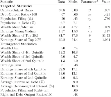
of the filing rate, are from Chatterjee et al. (2007). The targeted filing rate, .50%, is in the middle of the range used in the literature. Information on the

computation is in Appendix C.

The results from the calibration are listed in Table 1. The model does very

well at reproducing both the debt and filing targets as well as the earnings and

wealth targets. This is contrast to most of the bankruptcy literature, and the

discrepancy is mostly due to the flexible nature of the default cost. One less

attractive part of the calibration is that the right-tail households hold about

two-thirds of the total debt. These households have received below average

realizations of v, and so have had some incentive to borrow.

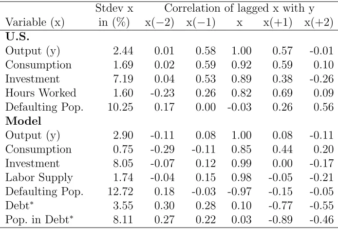
The model has untargeted predictions about cyclical properties, which are

reported in Table 2. The data are described in Appendix B. Filings are much

too countercyclical. However, as mentioned in the introduction, the filing rate

Statistic Data Model Parameter* Value

Targeted Statistics

Capital-Output Ratio 3.08 3.08 β .957

Debt-Output Ratio×100 .67 .66 χ0 .421

Population Filing (%) .50 .45 χ1 .730

Population in Debt (%) 6.7 7.1

Wealth Mean/Median 4.03 4.77 ξ .059

Earnings Mean/Median 1.57 1.53 πrl .147

Wealth Share of Top 20% 81.7 77.6 υ¯ 51.73

Earnings Share of Top 20% 60.2 54.4 υ 1.064

Untargeted Statistics

Wealth Gini .80 .74

Wealth Share of 4th Quintile 12.2 16.8

Wealth Share of 3rd Quintile 5.0 4.7

Wealth Share of 2nd Quintile 1.3 1.0

Earnings Gini .61 .48

Earnings Share of 4th Quintile 22.9 17.1 Earnings Share of 3rd Quintile 13.0 13.1 Earnings Share of 2nd Quintile 4.0 9.3

Average Interest on Debt (%) 9.0

Average Debt-weighted Interest (%) 16.3

Population Filing and Right-tail .00

Right-tail Debt-Output Ratio×100 .48

*Parameters are listed beside statistics they strongly influence.

to 2004 (-.94). Also, since default in the model is based entirely on earnings

shocks rather than (presumably) less cyclical reasons such as divorce, health

bills, and lawsuits, the model’s filing rate should be more countercyclical than

the data’s. Consumption exhibits excess smoothness. Output and investment

volatility are close to their U.S. counterparts. The correlations with output

are off, including the autocorrelation. Part of this failure is due to only having

two states for TFP.

Stdev x Correlation of lagged x with y Variable (x) in (%) x(−2) x(−1) x x(+1) x(+2)

U.S.

Output (y) 2.44 0.01 0.58 1.00 0.57 -0.01

Consumption 1.69 0.02 0.59 0.92 0.59 0.10

Investment 7.19 0.04 0.53 0.89 0.38 -0.26

Hours Worked 1.60 -0.23 0.26 0.82 0.69 0.09

Defaulting Pop. 10.25 0.17 0.00 -0.03 0.26 0.56

Model

Output (y) 2.90 -0.11 0.08 1.00 0.08 -0.11

Consumption 0.75 -0.29 -0.11 0.85 0.44 0.20

Investment 8.05 -0.07 0.12 0.99 0.00 -0.17

Labor Supply 1.74 -0.04 0.15 0.98 -0.05 -0.21

Defaulting Pop. 12.72 0.18 -0.03 -0.97 -0.15 -0.05

Debt∗ 3.55 0.30 0.28 0.10 -0.77 -0.55

Pop. in Debt∗ 8.11 0.27 0.22 0.03 -0.89 -0.46

*Debt is negative net worth.

Table 2: Business Cycle Properties: Model and Data (1960-2004)

4

Eliminating Default

I now explore the consequences of eliminating default both in terms of welfare

and allocations, and see how these change in the presence of aggregate risk.15

15_{I do not account for transitions. The main reason for this is computational. However,}

The benchmark economy, i.e. the one with consumer default, is referred to

as the CD economy. The economy with no default is referred to as the ND

economy. The ND economy is in fact just a “natural borrowing limit” economy

(see Aiyagari, 1994) where households are able to borrow, at a risk-free rate,

as much as they can repay with certainty.

While in most studies the use of a natural borrowing limit rather than some

exogenously fixed limit is of secondary importance, here it is the consequence

of eliminating default. Consequently, the natural limit is extremely important.

There are then three issues to consider, namely, what is the limit in the theory,

in the computation, and in the data. In the theory, the use of a log-efficiency process implies efficiency, and hence labor income, can be arbitrarily close to

zero prior to retirement. However, because some labor income isguaranteed in

retirement, the natural limit will not be zero as long as κG >0. In the

com-putation, the log process is discretized using a large support.16 _{This makes}

the lowest efficiency realization prior to retirement, .011, close to zero. In the

data, Carroll (1992) documents that non-capital household income, including

transfer income, falls to (or very close to) zero between .30% and .65% of the

time for working-age households. At the same time, part of Social Security

income, in particular Supplemental Security Income, seems to be guaranteed. Consistent with the data, the process I use has near-zero-earnings events but

allows for guaranteed earnings in retirement in both the theory and

compu-tation. Robustness tests are conducted with respect to the lower bound on

efficiency (see Appendix D).

4.1

Effects on Allocations

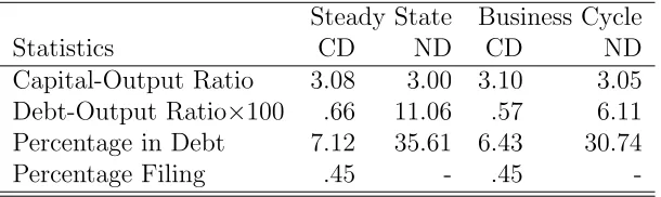
With or without aggregate risk, eliminating default results in a significantly

lower capital-output ratio and a very large increase in debt. This is borne

be seen shortly, eliminating default results in larger capital decumulation without aggregate risk than with it. Consequently, transitional dynamics are likely to strengthen the result that aggregate risk reduces the welfare gain of eliminating default.

16_{Specifically, the support is±6.25¯σ}

η,1/

p

1−¯γ2_{for the persistent shock and±5¯σ}

εfor the

out in Table 3 which lists statistics for both models (averages are presented

for the business cycle). However, another readily evident fact from Table 3 is

that eliminating default has a significantly smaller impact if one accounts for

aggregate risk. For instance, the debt-output ratio that before increased 1700%

(from .0066 to .11) now increases “only” 1100% (from .0057 to .0611). Another

way to interpret this result is that additional risk from the business cycle, and

the precautionary savings associated with it, has a much larger impact on the

ND economy than the CD one. In fact, the usual metric for precautionary

savings, the capital-output ratio, increases by 1.74% in the ND economy (3.00

to 3.05) but only by .55% in the CD economy (3.08 to 3.10).

Steady State Business Cycle

Statistics CD ND CD ND

Capital-Output Ratio 3.08 3.00 3.10 3.05

Debt-Output Ratio×100 .66 11.06 .57 6.11

Percentage in Debt 7.12 35.61 6.43 30.74

Percentage Filing .45 - .45

-Table 3: Eliminating default, with and without Aggregate Risk

This raises two questions. First, why is there so much more debt once

de-fault has been eliminated? Second, why is this effect reduced by aggregate risk?

The basic answer to these questions is that because of earnings uncertainty,

impatience, and a hump-shaped earnings profile, households in both economies

haveincentive to borrow. However, only the ND economy gives households the

opportunity to borrow large amounts, and this opportunity is diminished by

the inclusion of aggregate risk.

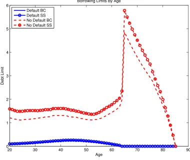
The best way to see this is to consider borrowing limits. While there is

no “borrowing limit” in the CD economy, there is an endogenous maximum

loan size that can be taken out by a household of type s: maxa0(q_g(a0, s;S) + qb(a0, s;S))(−a0). Similarly, no household in the ND economy would take out a

loan worth more than (¯qB(S)ρs)(−A¯(s;S)) where ¯A is the natural borrowing

limit (for type s in state S) and ¯qB = ¯qg + ¯qb is the no-arbitrage price of

averaging out the other components of s as well as S.17 _{One unit on the}

vertical axis can be equated to roughly $50,000.18 _{As is clear, the maximum}

loan size in the ND economy is uniformly and typically much higher than in

the CD economy. Because of this, and because households have incentive to

use debt, the ND economy is much more indebted. However, aggregate risk

noticeably reduces the natural borrowing limit, while leaving the CD limit

virtually unchanged. This reduces debt usage in the ND economy more than

in the CD economy.

20 30 40 50 60 70 80 90

0 1 2 3 4 5 6

Age

Debt Limit

Borrowing Limits By Age

Default BC Default SS No Default BC No Default SS

Figure 1: Borrowing Limits in the Default and No Default Economies

17_{This is done in the same as the welfare calculations, see Appendix C for details.}

18_{The averageeis normalized to one. The wage in the CD economy is roughly 1.2, and so}

While Figure 1 answers two questions, it raises two others: why do the

borrowing limits have such different shapes, and why does the natural

bor-rowing limit contract? Both answers lie in that the limits are determined by

completely different factors: whereas the CD limit is determined by household

willingness to repay onaverage, the ND limit is determined by household

abil-ity to repay in theworst circumstances. As it turns out, the minimum ability

of households to repay is larger than their average willingness, but it is also

reduced more by aggregate risk.

To see this, first consider the CD economy. There, the price of a bond is

determined by

q(a0, s;S) =X

z0 ¯

qz0(S)ρ_sEs,S,S0

z0(1−d(a

0

, e0, s0,0;S_z00)) and (24)

d(a, e, s,0;S) =1[VR(a, e, s,0;S)≥VD(e, s,0;S)] (25)

In these two equations one sees the average willingness to repay: the average

comes in the expectation overe0,s0, and—for ¯qz0 ≈q¯_BF(z0|z) implying a small equity premium—z0 as well; the willingness comes from the indicator function which states the value of repaying must be greater than the value of default.

Why is credit in the CD economy not affected much by the business cycle?

The primary reason is that recessions are short-lived. Because default rates are

very countercyclical (see Table3), if it were known that next period would be a

recession, credit would be very expensive:_Es,S,B(1−d) is close to zero, and for

a small equity premium the bond price would beq ≈q¯BEs,S,B(1−d). However,

since business cycles last for a relatively short time, the price households pay

reflects both a decreased willingness to pay in recessions (resulting in a low value for _Es,S,B(1− d)) and an increased willingness to pay in expansions

(resulting in a high value for_Es,S,G(1−d)). Consequently, they pay an “average”

price with q ≈ q¯BF(g|z)Es,S,G(1−d) + ¯qBF(b|z)Es,S,B(1−d). In fact, since

F(z0|z) is not far from 1/2, q≈q¯BEs,S(1−d) which is the steady state

aggregate risk.19

Now consider the ND economy. There, the borrowing limit can be

mechan-ically calculated as the net present value of future earnings. For a newborn

household, the formulas with and without aggregate risk are

Steady State

min

{st}

T

X

t=2

(

t−1 Y

j=2

¯ q∗_Bρsj)w

∗

e_st

s.t. F(st+1|st)>0

s1 given

Business Cycle

min

{st,zt}

T

X

t=2

(

t−1 Y

j=2

qB(Sj)ρsj)w(St)est,zt

s.t. F(st+1|st, zt+1)>0

St+1 = Γ(zt+1,St), s1,S1 given

(26)

where ¯q_B∗ andw∗are the steady state prices ande_xdenotes the lowest efficiency conditional onx.20As these definitions make clear, three factors can make the

limit decrease: changes in the support of e, changes in the support of s, and

changes in prices. The support of e changes in the business cycle because of

the labor supply shifterψz. Specifically,ψb =.977 causes the limit to decrease

by 2.3%. The support of s also changes slightly due to numerical precision,

specifically rounding in the normal cdf computation. However, by process of

elimination, the factor prices must account for most of the change.

Is it possible that the principal reason for the decline in the natural

bor-rowing limit is changes in factor prices? To check this, consider how the net

present value of guaranteed retirement income, a substantial contributor to the

natural limit, changes for young households in the deepest possible recession:

P85

t=46(

Qt−1

j=2q¯B(S)ρsj)w(S)κG

P85

t=46(

Qt−1

j=2q¯

∗

Bρsj)w

∗_κ

G

= .431

.789 =.55 (27)

19_{There could also be differences coming from factor prices, namely how the volatility}

(and slight changes in levels) of factor prices affect ¯qB and the average default decision

Es,Sd. However, these effects are fairly small.

20_{A technical point: these formulas assume thata}0 _{can be chosen from a continuum. Ifa}0

whereS reflectsz =band the lowestK/N possible for allt, andwand ¯qB are

the steady state values. Clearly, the decline is large: 45%. A key feature here

is that in a protracted recession, capital decumulation causes bothw and qto

decline. This lowers the natural limit for any age but especially so for young

households because the decline in q is compounded.

It is worth briefly interpreting this result. When default is eliminated,

cred-itors extend any amount of debt at a risk-free rate. While credcred-itors offer any

amount, households avoid taking on debt beyond what they can repay in the

worst case scenario. Absent aggregate risk, the worst case scenario is bad

ef-ficiency shocks forever. With aggregate risk, the possibility of a protracted recession makes the worst case scenario worse: households must now be

pre-pared for the worst efficiency shocks and the worst wages and the highest

interest rates (lowest bond prices). This is the why the natural limit contracts.

Not surprisingly, the differences in credit, prices, and default impact

con-sumption smoothing as seen in Figure 2 which plots the mean and variance

of log consumption from ages 20 to 30. For these young households, the mean

is always higher and the variance is always lower in the ND economies. This

is consistent with the ND borrowing limits always being greater than the CD

limits. However, the differences are less substantial with aggregate risk, which is consistent with the contraction in the natural limit. Lastly, the CD

econ-omy profiles from steady state look almost identical to the business cycle ones,

again in agreement with the CD borrowing limits changing little.

4.2

Welfare Effects

Eliminating default results in a large increase in debt and improved

consump-tion smoothing, but these effects are less pronounced with aggregate risk. I

now measure the welfare gain of eliminating default absent aggregate risk, and

see how including aggregate risk changes it.

The welfare measure I use is the percent increase in consumption that

20 21 22 23 24 25 26 27 28 29 30 −0.6 −0.5 −0.4 −0.3 −0.2 −0.1

Average of Log Consumption

Age

E(log(c)|age)

Default, Business Cycle Default, Steady State No Default, Business Cycle No Default, Steady State

20 21 22 23 24 25 26 27 28 29 30

0.04 0.06 0.08 0.1 0.12 0.14 0.16 0.18 0.2 0.22 Age Var(log(c)|age))

Variance of Log Consumption

Default, Business Cycle Default, Steady State No Default, Business Cycle No Default, Steady State

Figure 2: Mean and Variance of Log Consumption by Age

This is the same welfare measure used inLivshits et al. (2007),Athreya et al.

(2009b), and many others. Forσ = 2, this is

ω=

R

S

R

e,sVCD(0, e, s,0;S)dFˆ(e, s|z)dGCD(S)

R

S

R

e,sVN D(0, e, s,0;S)dFˆ(e, s|z)dGN D(S)

−1 (28)

where GX is the implied ergodic distribution over S induced by household

policies and stochastic transitions (includingz which is part ofS) in economy

X. While G could be a complicated object, its computational equivalent is

straightforward to calculate.21 _{If ω > 0, then eliminating default is welfare}

improving. For a more complete picture of the welfare effects, I also report the

percentage of the population in favor of the policy change and welfare gains

for other subsets of the population with details about these measures provided

in Appendix C.

Table 4 reports the welfare gains of eliminating default. Consistent with

the literature, eliminating default results in a large welfare gain of 3.78% for

21_{The computation in steady state is trivial since G puts all its weight on the steady}

stateS. In the business cycle, the method ofKrusell and Smith(1998) is used, and soS is summarized by z and m where m are moments of µ. The long-run distribution over m is then constructed using the approximate law of motion (see Appendix C for more details). If

R

e,sVCD(0, e, s,0;S)dFˆ(e, s|z)/

R

e,sVN D(0, e, s,0;S)dFˆ(e, s|z)−1 is computed at each point

young households absent aggregate risk. However, accounting for aggregate risk

reduces this by 1.05% to 2.73%. This is the first main finding of the paper,

and it agrees with the impact of aggregate risk on credit and consumption

smoothing.

While there is a large welfare gain for young households, only around 60%

of the population favor the policy change. The reason for the disagreement is

almost completely due to changes in factor prices. To isolate this effect, I also

present the welfare gains that would occur in partial equilibrium, i.e. holding

fixed the law of motion and prices r, w, ¯qg, and ¯qb. In partial equilibrium,

there is near unanimous support for eliminating default. Moreover, the welfare gain is much larger without aggregate risk, but the drop is also much larger

at 2.10% (moving from 6.00% to 3.90%).

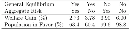
General Equilibrium Yes Yes No No

Aggregate Risk Yes No Yes No

Welfare Gain (%) 2.73 3.78 3.90 6.00 Population in Favor (%) 63.4 60.4 99.6 98.8

Table 4: Welfare Gains of Eliminating Default

To aid understanding of how these gains are distributed over the life cycle,

Figure 3plots average gains by age. To disentangle the effects of the changes

in credit from the changes in factor prices, consider first the gains in partial

equilibrium. The gains begin high for young households, decline monotonically,

and approach zero in retirement. The monotonic decline is due to diminishing

incentives for borrowing: young households have life-cycle reasons to borrow

and face uncertainty, middle-aged households have only uncertainty, and

re-tired households have neither. Additionally, aggregate risk causes a uniform decline in the gains with the largest drops occurring for young households.

This shows the effect of credit becoming less effective in the ND economy.

Now consider general equilibrium. As before, young households experience

a significant welfare decline from eliminating default, although the drop is less

have the opposite experience. The changes relative to partial equilibrium are

due to the relative importance of wages verse interest rates over the lifecycle.

Young households are wealth poor and prefer a larger capital-output ratio since

it has higher wages (although this desire is tempered by a desire to borrow

at low interest rates). Older households, who derive much of their income

from assets, favor a smaller capital-output ratio with the associated increase

in interest income.

20 30 40 50 60 70 80 90

−1 0 1 2 3 4 5 6

Age

Consumption Gain (%)

Consumption Gain of Eliminating Default by Age

Business Cycle, General Eq Steady State, General Eq Business Cycle Partial Eq Steady State, Partial Eq

5

Restricting Default

The previous section analyzed how aggregate risk affected the consequences

of eliminating default. I now consider how aggregate risk affects the

conse-quences of restricting default, looking at high, but not infinite, default cost

regimes, the Bankruptcy Abuse Prevention and Consumer Protection Act of

2005 (BAPCPA), andz-contingent default policies.

5.1

High, but not Infinite, Default Cost Regimes

One might be tempted to conclude the welfare loss and contraction of credit

in the ND economy occur because the natural borrowing limit is a special case where default is infinitely costly, i.e. one in which χ(e) = 1. However,

aggregate risk also causes economies with large—but not infinite—default costs

to experience similar contractions of credit and reductions in welfare. This is

seen in Table 5 which reports the effects of moving from the CD economy to

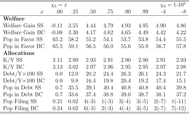
economies with differing levels of χ0. For easy interpretation, the progressive

component,χ1, has been fixed at zero. The infinite default cost economy (ND)

is χ0 = 1.

The business cycle reduces the welfare gain, debt-output ratio, and

popu-lation in debt for each computed level ofχ0 >0. This effect tends to increase

in χ0 with the χ0 > .9 regimes experiencing the largest declines. Moreover,

the regime with the highest welfare gain in steady state is χ0 = .99 while in

the business cycle it is lower at .90. These results show that the qualitative

features from making default infinitely costly extend to the case of making it

very costly.

Why does this result obtain? Consider first the following. Because

house-hold’s can always choose a0_g = a0_b = 0, a lower bound on the value of default (ignoring mortality risk) is_Et

P

τ≥tβ

τ−t_u(w

τeτ(1−χ0)). Forσ= 2, this can be

written as (1−χ0)−1EtP_τ≥tβ

τ−t_u(w

τeτ). Now suppose that, because default

is costly, a household wants to limit their exposure by not defaulting more

than π amount of the time. Then the expected utility loss from default is not

more than π(1−χ0)−1EtP_τ≥tβ

τ−t_u(w

χ0 =x χ0 = 1-10x

x .00 .25 .50 .75 .90 .99 -4 -8

Welfare

Welfare Gain SS -0.11 3.55 4.44 4.79 4.93 4.95 4.90 4.86 Welfare Gain BC -0.08 3.30 4.17 4.62 4.65 4.49 4.42 4.22 Pop in Favor SS 65.2 58.2 55.2 54.1 53.7 53.8 54.4 55.5 Pop in Favor BC 65.5 59.1 56.5 56.0 55.6 55.9 56.7 57.8

Allocations

K/Y SS 3.11 2.99 2.93 2.91 2.90 2.90 2.91 2.93

K/Y BC 3.13 3.02 2.97 2.96 2.95 2.95 2.97 2.98

Debt/Y×100 SS 0.0 12.0 20.2 24.4 26.3 26.1 24.3 21.7

Debt/Y×100 BC 0.0 9.8 16.4 19.8 20.4 19.2 17.4 15.1

Pop in Debt SS 0.7 35.5 39.1 40.4 40.8 40.8 40.4 39.8

Pop in Debt BC 0.7 33.6 37.4 38.8 39.0 38.7 38.1 37.2

Pop Filing SS 0.21 0.02 4(-3) 1(-3) 3(-4) 3(-5) 2(-7) 1(-11) Pop Filing BC 0.24 0.02 6(-3) 2(-3) 4(-4) 3(-5) 2(-7) 7(-12) Note: SS means “steady state” and BC means “business cycle.”

Forχ0 = 1−10−20, the results are the same as ND, including no default.

Notationa(b) meansa × 10b.

Table 5: Welfare Gains of Making Default More Costly

such that π(1−χ0)−1 is constant protects the household—in expected utility

terms—from default. In fact, this is what Table 5 suggests is happening: as the default cost increases, it is met with a corresponding decrease in default

rates.

Finally, note that to only default π amount of the time, households must

limit the amount of debt they take on. When π = 0, this is the natural

bor-rowing limit from the ND economy. However, when π ≈0, this is close to the

natural borrowing limit. Consequently, when aggregate risk makes the natural

borrowing limit contract, it causes the borrowing limit implied by π ≈ 0 to

also contract. This is why the results when default costs are large are similar

to when default costs are infinite.

It is also worth pointing out that the welfare gains from relatively low values

risk, this occurs here for χ0 = .5 which results in a welfare gain of 4.44%

compared to eliminating default with a gain of 3.78%. With aggregate risk,

a lower value of χ0 = .25 results in a welfare gain of 3.30% compared to the

gain from eliminating default of 2.73%. Hence, if one were to try to improve

bankruptcy law, one need not go to a very high default cost regime—especially

when considering aggregate risk.

5.2

BAPCPA

The Bankruptcy Abuse Prevention and Consumer Protection Act of 2005

(BAPCPA) is an important example of restricting default. Among many other

changes (see White, 2007, for a comprehensive list), the reform has made it

typically impossible for households with above median income in their state to file for Chapter 7 bankruptcy. At the same time, it did not eliminate debt

forgiveness for these households because they may still file for Chapter 13.

This chapter of the bankruptcy code allows households to obtain partial debt

forgiveness by forfeiting future income for three to five years (with the benefit

being that households may keep their assets).

This legal environment is mapped into the model in the following way. First,

households with efficiency less than ψze˜, where ˜e is the median efficiency in

steady state, may default as before. Second, households with efficiency above

ψz˜e may forfeit a fraction χ13 of their earnings to creditors in the period of

default in exchange for all their debt. They subsequently enter into bad

stand-ing (h = 1) with a zero net asset position. When χ13 is paid, this replaces

the default cost χ(e) in the period of filing.22 _{I set χ}

13=.75 to loosely

repre-22_{These assumptions alter repayment probabilities,}

p(a, s−1;S) =Es−1,S

1 +d(a, e, s,0;S)

−1 +1e>ψze˜

χ13w(S)e

−a

,

and consequently affect contract pricing via (13) and theK0 calculation via (18). A similar adjustment must be made for computing capitalK,

K(S) =

R

a1 +d(a, e, s, h;S)−1 +1e>ψze˜

χ13w(S)e −a

dµ

sent a 15% annual contribution of earnings over the course of 5 years.23 _While

there are much better ways of modeling Chapter 13 bankruptcy (a good

ex-ample being Li and Sarte, 2006), this formulation captures the quintessential

feature of Chapter 13 that debt is forgiven in exchange for income without

overcomplicating the model.

What are the positive effects of BAPCPA? Table 6 reports the

capital-output ratio and debt and filing statistics after the policy change alongside

their CD and ND counterparts. Surprisingly, BAPCPA increases total filings

by .20 percentage points. Moreover, despite this increase in default, the

equi-librium level of debt and population in debt are both substantially larger. How-ever, as one might expect, BAPCPA significantly reduces default by

above-median earnings households. This effect is so strong it virtually eliminates

filings by these households.24

To understand these effects, it is useful to look again at the average

bor-rowing limits. These are plotted in Figure 4 for the BAPCPA, CD and ND

economies. The most striking feature is that credit expands the most for

middle-aged households resulting in the BAPCPA limit having a more

pro-nounced hump than the CD limit. In fact, the increase makes the BAPCPA

borrowing limits larger than the natural borrowing limit for some households. It is also clear that the BAPCPA reform borrowing limits are affected only

slightly by aggregate risk.

Why does the reform cause credit to expand, and why is this effect strongest

23_{In the law, households in this situation would have to contribute 100% of “disposable}

income,” income exceeding allowances defined by the IRS, for 5 years. For a two person household these allowances can exceed $17,500.

24_{It is good to ask whether the model’s predictions correspond to the data. Unfortunately,}

Debt/Y % Filing

Economy K/Y ×100 % in Debt % Filing e≤ψze˜

Steady State

CD 3.08 0.66 7.12 0.45 0.31

ND 3.00 11.06 35.61 0.00 0.00

BAPCPA 3.05 2.18 12.35 0.65 0.65

Business Cycle

CD 3.10 0.57 6.43 0.45 0.32

ND 3.05 6.11 30.74 0.00 0.00

BAPCPA 3.07 2.04 11.41 0.65 0.65

CDR∗ 3.11 0.25 7.62 0.34 0.27

CDE∗ 3.12 0.18 7.63 0.14 0.11

∗

These aggregate-state contingent policies have no steady state.

Table 6: Effects of Restricting Default on Allocations

for middle-aged households? The answer is straightforward: the median

effi-ciency test, paired with a shaped earnings profile, results in a hump-shaped average default cost. This hump-hump-shaped average default cost is seen

not only in borrowing limits, but also in the lifecycle paths of debt and default,

which are displayed in Figure 5. As default costs increase towards middle-age,

so does the population in debt and the average level of debt held by a debtor.

Somewhat surprisingly, so do filings. As was seen in Table 6, these defaults

are virtually all by below median households. What is occurring then is that

households become encumbered by debt while above median or just below

median income (for them debt is cheap since they face high default costs in

expectation) and subsequently default when their income falls.

An important but less obvious feature in Figure 4 is how aggregate risk

causes the debt limit to contract in the BAPCPA economy. The only

dis-cernible contraction is seen for middle-aged households, for whom the

median-earnings restriction tends to bind. Consistent with the findings for the high

default-cost regimes in Table 5, the business cycle causes credit to contract

when default is costly. However, here, default is only more costly for the

20 30 40 50 60 70 80 90 0

1 2 3 4 5 6

Age

Debt Limit

Borrowing Limits By Age

Default BAPCPA BC Default BAPCPA SS Default BC

Default SS No Default BC No Default SS

Figure 4: Borrowing Limits with the BAPCPA Reform

aggregate risk while credit for other households is roughly unchanged.

Did restricting default through BAPCPA improve welfare? The models with and without aggregate uncertainty suggest a small welfare loss (-.06%

with and -.07% without) for newborn households with 56% of the population

opposed to the change (with or without aggregate risk). In contrast, the partial

equilibrium welfare losses are gains of .39% with and .38% without aggregate

risk, and the population almost unanimously prefers it at 99.1% and 99.9%

respectively.

Given the preceding discussion, these results are easily explained. BAPCPA

causes a significant expansion in credit for middle-aged households but only a

20 30 40 50 60 70 80 0

10 20 30

Population in Debt

Population (%)

CD BAPCPA

20 30 40 50 60 70 80

0.1 0.2 0.3 0.4 0.5

Debt conditional on being a debtor

Debt

20 30 40 50 60 70 80

0 1 2

Default Rate

Defaults (%)

age

Figure 5: Lifecycle Profiles of Debt and Default Absent Aggregate Risk

households prefer this expansion. However, since the ability for young

house-holds to borrow is only marginally increased, there is only a small welfare

gain for young households. When one adds the general equilibrium effects

lower wages and higher interest rates due to less capital, this small welfare

gain becomes a small welfare loss, and there is more disagreement because the

importance of wages and interest rates vary over the business cycle. Lastly,

aggregate risk only causes a noticeable contraction in credit for middle-aged

5.3

Aggregate-State Contingent Default Policy

I now consider a different type of default restriction that allows default only in

recessions or, for completeness, only in expansions. This is meant to capture

the pattern of legislation responding to negative aggregate shocks with more

debt forgiveness and to positive shocks with less. The policy that allows default

in recessions (z = b) is referred to as CDR; the policy where default is only allowed in expansions (z =g) is referred to as CDE.

A priori, one might expect that either economy would look like a convex

combination of the CD and ND economies. Surprisingly, the aggregate

statis-tics reported in Table6do not bear this out. In particular, the CDR and CDE

economies have the highest capital-output ratio and the least amount of debt.

The proximate cause of this lack of debt is revealed in Figure 6which plots

borrowing limits for the CD, ND, CDR, and CDE economies. In the CDR and

CDE economies, the borrowing limits for newborn households lie below the

CD economy’s limit until age 61. Additionally, the borrowing limits are much less than but have the same shape as the ND economy limit.

To understand why the CDR and CDE limits are tight prior to retirement

and have the same shape as the ND limit, consider CDR (the logic is the

same for CDE). In this case, there exists one possible scenario, expansion for

a lifetime, where households will never be allowed to default. Consequently,

a natural borrowing limit (like the ND limit) is in effect because—to ensure

consumption is nonnegative—households must not borrow more than the net

present value of the lowest possible earnings stream conditional on this

se-quence of aggregate shocks.

Now consider how this natural limit, which is different from the usual

one, is determined. Since households with the lowest possible earnings stream

(let s denote the associated s) are very prone to default if a recession

oc-curs, p(a0, s;B) ≈ 0 for most levels of debt. Hence, qb(a0, s;S) ≈ 0. Since

households are not allowed to default in G, qg(a0, s;S) = ¯qg(S). These

obser-vations, together with a small equity premium giving ¯qg(S) ≈ q¯B(S)F(g|z),

imply qg(a0, s,S) +qb(a0, s,S) ≈ q¯B(S)F(g|z). This is less than or equal to

¯

20 30 40 50 60 70 80 0

0.2 0.4 0.6 0.8 1 1.2 1.4 1.6 1.8

Age

Debt Limit

Borrowing Limits By Age

Default Recessions Only Default Expansions Only Default

No Default

Figure 6: Borrowing Limits with Default in Recessions or Expansions Only

Because households with the worst earnings stream face this low price (high

interest rate), the net present value of the worst earnings stream is drastically lowered: a unit of labor income from age 65 is worth roughly .4 = .9845 _at

age 20 when discounted by ¯qB(S); this drops to .5×10−8 = (.98·2/3)45 when

discounted by ¯qB(S)· 2/3. Because future earnings are discounted heavily,

the limit in the CDR economy is very tight. This reasoning is verified by

the observation that, as age 85 approaches, the CDR and CDE borrowing

limits approach the ND limit—discounting ceases to matter since all future

guaranteed earnings are just a few years away.

Given the tight borrowing constraints, one might expect that both the