A Collaborated Multi-controller Strategy by Using L1 Adaptive Augmentation
Control for Power-generation Systems with Uncertainties
Lei Pan, Jiong Shen
Southeast University, School of Energy and Environment,
Key Laboratory of Energy Thermal Conversion and Control of Ministry of Education, Si Pai Lou Str. 2, 210096 Nanjing, China
e-mail: [email protected], [email protected]
Chengyu Cao
University of Connecticut, Department of Mechanical Engineering, Auditorium Rd. 191, Storrs, CT 06269-3139, USA
e-mail: [email protected]
http://dx.doi.org/10.5755/j01.itc.44.3.8846
Abstract. For dealing with uncertain operation circumstances, a collaborated multi-controller strategy of the cascade architecture with a L1 adaptive augmentation controller and a conventional baseline controller is introduced to
power-generation systems. For its arbitrarily close, fast, and robust tracking performance, the L1 adaptive output
feedback controller is designed as the augmentation controller in the inner-loop to keep the nominal dynamics of the system in the overall operation scope. The robust PID controller and offset-free linear MPC controller are recommended as the available outer-loop baseline controllers to follow control commands. The closed-loop stability of the cascade control system is ensured. The simulation experiments on a benchmark nonlinear boiler-turbine generation model verify the greatly improved adaptation and robustness of the augmentation control system in the presence of unknown uncertainties. Additionally, it is easy to upgrade a conventional control system to this cascade one in practice because the add-in L1 adaptive augmentation controller influences little on the augmented system setup.
Keywords: L1 adaptive controller; linear controller; uncertainty; nonlinearity; power plants.
1. Introduction
Nowadays, power-generation units inevitably operate in uncertain circumstances due to the disturbances caused by the intermittent emission control, the fluctuations of lower heating value (LHV) of fuel and the uncertain power supply by other renewable energy in grids. Their existing control systems usually cannot handle these uncertainty issues well and may lead to unstable operations. No doubt it is significant for power plants to improve the adaptation and robustness of their controllers for dealing with unknown uncertain conditions.
There are many control approaches in literatures on handling disturbances and modeling mismatch. A general state-space disturbance model is presented in [1] for the linear model predictive control (MPC). Based on the detectability conditions of the augmented disturbance model, steady-state offset
with Uncertainties
having nonlinearities, time-varying disturbances, unknown parameters and un-modeled dynamics. Therefore, we have studied the L1 adaptive control strategy for the nonlinear boiler-turbine systems with internal un-modeled dynamics, time-varying parameters and unknown disturbances in our previous work [9], which shows that the proposed L1 adaptive controller guarantees good control quality for the power generation process in the presence of unknown uncertainties.
However, it may be unrealistic to fulfill the L1
adaptive controllers independently in large-scale power units. Because there are many coupled chemical loops in such sophisticated thermodynamic systems, it is difficult to replace all the conventional controllers by the novel advanced controllers. One feasible way is to augment the L1 adaptive controller into the conventional control systems for dealing with unknown uncertainties. This augmentation control strategy may be more reliable with less parameter modifications on the existing control systems to obtain a better control quality and thus has great practical significance. Therefore, we propose a collaborated multi-controller strategy for power-unit systems with severe nonlinearity, bounded disturbances and unknown uncertainties in this paper, i.e. the approach of the L1 adaptive augmentation controller collaborating with baseline controllers like PID or MPC. In this strategy, the L1 adaptive controller is augmented as an inner-loop controller in cascade with the baseline controller for compensating all the unknown disturbances and uncertainties. Among many kinds of L1 adaptive control methods, an extension approach of the L1 adaptive output feedback control [10] to systems of unknown relative degree is very suitable to make the augmentation controller. This approach adopts a new piece-wise continuous adaptive law along with the low-pass filtered control signal. It allows for achieving arbitrarily close tracking of the reference signals, and the transfer function of its reference system is not required to be strictly positive real. Stability of this system is guaranteed by its design via small-gain type argument. These features show that this L1 adaptive control approach may have great potential to be applied in wide industrial processes. Moreover, we will take two kinds of wide-applied baseline controllers for the augmented cascade-loop design and verifications, one is the robust PID controller; another is the offset-free linear MPC. We will make them to be augmented by the L1 adaptive output feedback controller and then to be used as the rapid coordinated tracking control system of the power-generation systems with severe nonlinearities, internal un-modeled dynamics, time-varying unknown disturbances and parameters.
In this collaborated multi-controller strategy, the
L1 adaptive augmentation controller and the baseline linear controller collaborate together but are independent in the algorithms and even in hardware.
Any existing controller in power units can be augmented by an inner-loop L1 adaptive controller to compensate the unknown uncertainties with little modifications on the existing controller parameters and then obtain enhanced control quality. It can be programmed in an independent controller from its partner linear controller, and only simple connections are made for them. Thus the L1 adaptive augmentation controller has great advantage for the real implementations.
The remainder of the paper is organized as follows. In Section 2, we propose the cascade control architecture and design the inner-loop L1 adaptive augmentation controller. In Section 3, a classic nonlinear boiler-turbine model is introduced for the study. In Section 4, two kinds of linear controllers with robust stability are introduced as the outer-loop baseline controllers. In Section 5, several simulation scenarios about wide-range load tracking with severe nonlinearity and unmatched model parameters are conducted to evaluate the performances of the collaborated multi-controller strategy of two kinds of baseline controllers and the L1 adaptive augmentation controller. In Section 6, we draw the conclusions for the study.
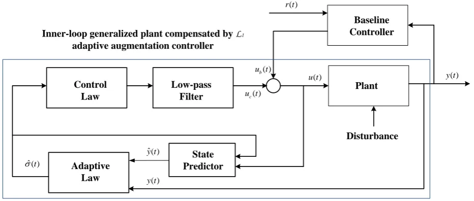
2. Cascade architecture of
L
1adaptive
augmentation controller and baseline
controller
The baseline controllers like PID and MPC are widely applied in power units. It has real significance for power stations to enhance their baseline controllers by augmenting L1 adaptiveoutput feedback controller to compensate nonlinearities, time-varying distur-bances, model mismatch and un-modeled dynamics in the power generation process. The augmentation control architecture is shown in Fig. 1.
In this architecture, the baseline controller is designed for one working point, usually the nominal point. The L1 adaptive augmentation controllers are used to maintain the desired system performance defined by the nominal baseline controller close-loop dynamics, in the presence of nonlinearities, time-varying disturbances, model mismatch and un-modeled dynamics in the overall operation range. Under this objective, the L1 adaptive augmentation controller uses a fast adaptation algorithm to estimate the un-modeled uncertainties, and then it outputs a band-limited augmentation control signal by its control law to compensate the disturbances and model mismatch from the nominal working point. The total control signal is
u(t) = ub(t) + uc(t) (1)
where ub(t) denotes the output of the baseline
controller, and uc(t) denotes the output of the L1
the baseline controller, the augmentation control signal produced by the L1 adaptive control law tends to zero.
L1 adaptive augmentation controller and the baseline controller are independent of each other in algorithms. The design of the L1 adaptive augmentation controller is presented in this section.
2.1. Problem formulation
We describe the controlled plant dynamics as follows:
0
0
( ) ( ) ( ) ( , , ), (0) , ( ) ( , , ), (0) ,
( ) ( )
m m
T m
x t A x t B u t f x z t x x z t g z x t z z
y t C x t
(2)
where x(t)Rn is the system state vector(measurable), u(t)Rm is the input vector(m≤n), y(t)Rm is the
output vector, Am Rnn is a known Hurwitz matrix, Bm Rnm is a known full-rank constant matrix, CmRmn is a known full-rank constant matrix, (Am, Bm, Cm) defines the desired dynamics for closed-loop
system, (Am, Bm) is controllable, (Am, Cm) is
observable, zeros of CmT(SI-Am)-1Bm lie in the open
left-half s plane, z(t)Rp is the immeasurable state
vector of internal un-modeled dynamics, and
: n p n
f R R R R and : n p p
g R R R R are
unknown nonlinear functions.
The control objective is to design an augmentation adaptive output feedback controller, u(t), such that the system output - y(t) - tracks the desired system output
ydes(t) with desired transient and asymptotic
performance. The desired system is described by
( ) ( ) ( ),
( ) ( )
des m des m des
T
des m des
x t A x t B u t
y t C x t
(3)
where (Am, Bm, Cm) represents the nominal dynamics
of the controlled plant in this approach.
2.2. L1 adaptive augmentation controller
L1 Adaptive controller consists of the state predictor, the adaptation law and the control law.
1) State predictor. Thestate predictor is given by:
0
ˆ( ) ˆ( ) ( ) ˆ( ) ˆ( ) ˆ( ), (0)ˆ
m m
T m
x t A x t B u t t
y t c x t x x
, (4)
where ˆ( )x t Rn and ˆ( )y t Rm are the state and output
of the predictor respectively; ˆ ( ) t Rn compensates
the system disturbances and model mismatch. We can find a constant matrix, n(n m)
um
B R , such that
0
T m um
B B and rank([Bm Bum]) = n. Then, equation (4)
can be written as
1 2
0
ˆ( ) ˆ( ) ( ( ) ˆ) ˆ , ˆ( ) ˆ( ), (0)ˆ
m m um
T m
x t A x t B u t B
y t c x t y y
(5)
where ˆ ( )1 t represents the matched component of
ˆ ( )t
, and ˆ ( )2 t represents the unmatched
component.
2) Adaptation law. ˆ ( ) t is on-line estimated by
the following adaptation law:
1
ˆ( ) ˆ( ) [ , ( 1) ], ˆ ( ) ( ) ( ), 0,1, 2,
t iT t iT i T
iT T iT i
(6)
where T>0 is the integration time of the adaptation law; and 1 1 ( ) 0 1 ( ) ,
( ) 1 ( ), 0,1, 2,
m
m
T A T
A T
T e d
iT e y iT i
(7)where 11 RN is the basis vector with first element 1 and all other elements zero;
ˆ
( ) ( ) ( ); ,
T
m N N
c
y t y t y t R
D P
where
P=PT>0 satisfies the algebraic Lyapunov equation
Baseline Controller Plant State Predictor Adaptive Law Control Law Low-pass Filter
ˆ ( )t
ˆ( ) y t ( ) y t ( ) u t ( ) r t Disturbance ( ) b u t ( ) c u t
Inner-loop generalized plant compensated by L1 adaptive augmentation controller
( ) y t
with Uncertainties
AmTP + PAm = -Q, Q > 0; and D R (N-1)Nsatisfies 1
( T( ) )T 0
m
D c P .
3) Control law. The control law is defined as follows: 1 1 2 ˆ ( ) ˆ [ ] ( ).
ˆ ( ) m um t
B B t
t
The augmentation control signal is given via the output of the low-pass filter C(s):
1 2
ˆ ˆ
( ) ( )( ( ) ( ) ( )),
c
u s C s s M s s (8)
where the L1 adaptive augmentation controller output
uc(t) is the inverse Laplace transform of uc(s); C(s)=KD(s)(Im+KD(s))−1 is a strictly-proper stable
low-pass filter matrix with DC gain C(0) = Im, K∈Rm×mis a gain matrix, D(s) is a m × m
strictly-proper transfer function matrix (the choice of K and
D(s) needs to ensure that C(s)M(s) is proper and stable), ˆ ( )1 s and ˆ ( )2 s are the Laplace
transformations ofˆ ( )1 t and ˆ ( )2 t , respectively. M(s)
is defined by
1
( ) ( mT( ) xm( )) ( mT( ) xum( )),
M s C s H s C s H s (9)
1 1
( ) ( ) ,
( ) ( ) .
xm n m m
xum n m um
H s SI A B
H s SI A B
(10)
The above piece-wise continuous adaptive law with the low-pass filtered control signal allows for achieving arbitrarily close tracking of the input and the output signals of the reference system. The performance bounds between the closed-loop reference system and the closed-loop L1 adaptive system can be rendered arbitrarily small by reducing the step size of integration. It can be represented by the following equations:
0 0
lim ( ) ref( ), lim ( ) ref( )
T y t y t T u t u t . (11)
The proof of the feasibility and stability of the above method can be found in [11].
Remark 1. With a fast-sampling L1 adaptive augmentation controller, all the disturbances and model-plant mismatch in the baseline controller loops can be estimated out and timely compensated, and thus the inner loop including L1 adaptive augmentation controller and the plant can perform a desired dynamics for the baseline controllers to control. The sampling time T should be small enough for L1
adaptive augmentation controller to achieve a timely compensation on the desired dynamics.
2.3. Closed-loop Stability
Assume that a precise compensation for the model mismatch is made by the L1 adaptive augmentation controller, namely the inner loop maintains the nominal dynamics in the presence of unknown uncertainties. Then the closed-loop stability and transient performance of the cascade system depends on the outer-loop baseline controller. It’s not difficult
to choose a stable linear controller, e.g. many PID controllers and stable MPC controllers.
Because the sampling frequency of the L1adaptive augmentation controller is much higher than that of the baseline controller, the stability of the inner loop is ensured by the L1 - gain stability condition [7] of the
L1 adaptive augmentation controller which can be satisfied by designing a proper filter. The tracking performance bounds between the desired dynamics and the inner-loop dynamics can be rendered arbitrarily small by reducing the integration step size of the L1 adaptive augmentation controller, the proof can be found in [8,11]. Therefore, one should make the sampling time T of the inner loop small enough so that the tracking bounds can be tolerated by the baseline controller in the sense of its stability margin.
In a word, the stability of the cascade system can be guaranteed by a L1 adaptive augmentation controller which satisfies the L1 - gain stability condition and its fast-sampling which makes the tracking bounds of the inner loop to the nominal dynamics small enough within the stability margin of a nominal stable baseline controller.
3. Dynamic model of a nonlinear
boiler-turbine-generator unit
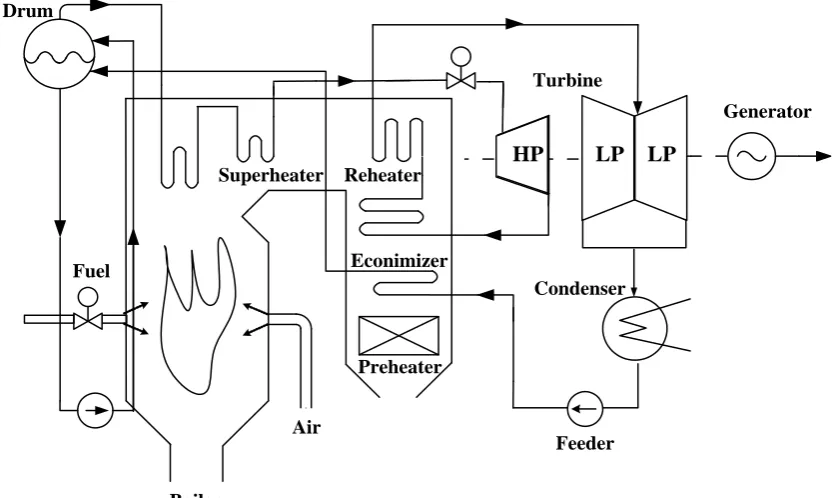
Before we design the L1 adaptive augmentation control system for power-generation units, we introduce the nonlinear boiler-turbine-generator unit model of Bell and Åström [12] to be the controlled plant in our study in this section. This model was derived specifically for a steam boiler with a turbine in a power plant unit. Due to its capability of capturing the key characteristics of real boiler-turbine systems, including multiple variables, nonlinearity, unmeasured internal state, strong coupling, large inertia, non-minimum phase, and unstable plant etc., this model has been widely used in literature as a benchmark for control studies [13-18], and has also been chosen by us for developing and verifying the L1 adaptive augmentation control approach. A schematic picture of the boiler–turbine system is shown in Fig. 2. The steam boiler part converts the input chemical energy of fuel into the thermal energy that is directly fed to the turbine part and is converted into the mechanical energy and then the electricity energy in the generator finally.
The model is a third-order multiple input multiple output nonlinear dynamic equation group, described as follows:
9 / 8
1 2 1 1 3
9 / 8
2 2 1 2
3 3 2 1
1 1
2 2
3 3
0.0018 0.9 0.15 (0.073 0.016) 0.1 [141 (1.1 0.19) ] / 85
0.05(0.1307 100 cs e/ 9 67.975)
x u x u u
x u x x
x u u x
y x
y x
y x a q
where the state variables are drum steam pressure x1 in units of kg/cm2, electric power x
2 in MW and drum/riser fluid density x3 in kg/cm3. The output variables y1 and y2 are the same as x1 and x2; the output y3 in units of meter denotes the drum water level deviation, where evaporation rate αcs in kg and steam quality qe in kg/s are given by
2 1 1 3
(0.854 0.147) 45.59 2.514 2.096 e
q u x u u , (13)
3 1
3 1
(1 0.001538 )(0.8 25.6) (1.0394 0.0012304 )
cs
x x
a
x x
. (14)
The input variables include the normalized fuel flow rate u1 (0-1 corresponds to 0-14kg/s), control valve position of steam to the turbine u2 (0-1) and normalized feedwater flow rate u3 (0-1 corresponds to 0-14kg/s). The inputs are subject to magnitude and rate saturations as follows:
0ui1,i1, 2, 3
1
0.007 u 0.007
2
2 u 0.002
3
0.005 u 0.05
. (15)
Its verified working points are shown in Table 1. The nominal one is marked as #2.
4.
L
1adaptive augmentation control system for
nonlinear boiler-turbine-generator units
Based on the cascade architecture of augmentation control shown in Fig. 1, we will design the L1adaptive
Table 1. Equilibrium operating points of the boiler-turbine dynamics
augmentation control system for the nonlinear boiler-turbine-generator unit. We take two typical kinds of controllers often used in the power plants to be the baseline controllers in the augmentation control system. One is the robust PID; another is the offset-free linear MPC (OFL-MPC). They are representative for the conventional control and the advanced control approaches, respectively.
4.1. L1 adaptive augmentation control system I: L1
adaptive controller and robust PID controller A robust PID controller in [13] has shown its good performance in the wide-range load-tracking process of the nonlinear boiler-turbine-generator model (12)-(15) and thus been well-known. It is designed from the loop-shaping H∞approach by using a linearized model
at the nominal operating point. A precompensator and postcompensator were designed with a constant decoupler, aligning the singular values of the model at 0.001 rad/s. The resulting H∞ controller is then
transformed into four SISO PI controllers by using a
Superheater
Turbine
Generator
Reheater
Econimizer
Preheater
HP
LP
LP
Fuel
Air
Boiler Drum
Feeder Condenser
Figure 2. Schematic of a boiler-turbine-generator unit
#1 #2 #3 #4
x1 75.6 108 129.6 135.4
x2 15.27 66.65 105.8 127
x3 299.6 428 513.6 556.4
u1 0.156 0.34 0.505 0.6
u2 0.483 0.69 0.828 0.8971
u3 0.183 0.433 0.663 0.793
with Uncertainties
PID reduction method. The anti-windup bumpless transfer (AWBT) technique is employed after the PID controller design to compensate for the effect of the constraints. The final form of the AWBT PI controllers will be easy for its real application. Here the PI controller has the form k(s) = k(1+1/lS) and the four
PI controllers are given by
0.0012 0.0486
0.0045
0.2914
0.0485 0 1.2091
( ) 0 0.0197 0
0 0 7.2548
s s
s
s
K s .(16)
The schematic of an anti-windup PI controller is shown in Fig. 3 [12].
Plant k
+
Disturbance
r K(s) y
l k 1 s 1 k
-Figure 3. One AWBP PI controller
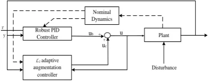
The AWBP PI controllers have very limited tolerance in parameter perturbations and disturbances. We enhance it with the L1 adaptive augmentation controller as shown in Fig. 4.
Plant Robust PID
Controller
Nominal Dynamics
L1 adaptive
augmentation controller ub + + Disturbance r y uc u
Figure 4.Robust PID and L1 adaptive augmentation
control scheme
4.2. L1 adaptive augmentation control system II: L1
adaptive controller and OFL-MPC
For achieving energy-saving and safe operation in the power-generation process, many PID controllers in power plants have been upgraded into MPC controllers due to their successfully solving the control problems with long delay, with coupled inputs and with constraint optimization. The OFL-MPC [1,2] is an efficient control approach in constrained linear processes for its performances on output tracking without steady-state offset, stability guarantee and disturbance rejections. But it cannot deal with the severe nonlinear dynamics and large model-plant mismatch. We introduce this approach in the following and then test its performance under unknown uncertain conditions without and with a L1 adaptive augmentation controller, respectively, in the simulations.
The OFL-MPC is composed of three components: an augmented observer with estimated disturbance signals, an online constrained target generator and an input-to-state stabilizing predictive controller. Its nominal plant model is the same as the desired model of the L1 adaptive augmentation controller, i.e.
( ) ( ) ( ), ( ) ( )
m m
T m
x t A x t B u t y t c x t
(17)
which is discretized into
( 1) ( ) ( )( ) ( )
x k Ax k Bu k
y k Cx k
. (18)
The OFL-MPC approach lumps the mismatch and disturbances into the augmented states to make a disturbance model as follows
( 1) ( )
( )
( 1) 0 1 ( ) 0
( )
( )
( )
.
x k A E x k B
u k
d k d k
x k
y C F
d k k
(19)The observability of the disturbance model (19) is given in Lemma 1[2].
Lemma 1. The disturbance model presented in (18) is detectable if and only if (C, A) is detectable and
( )
d
I A E
rank n n
C F
, (20)where n is the number of the nonaugmented states, nd is the number of the disturbances.
1. Augmented Observer. Consider the following observer
1
2
ˆ( 1) ˆ( )
ˆ
( ) [ ( ) ( )]
ˆ( 1) 0 ˆ( ) 0
ˆ( ) ˆ( )
ˆ( )
x k A E x k B L
u k y k y k
d k I d k L
x k
y k C F
d k (21)
where the observer gain [ 1 2]
T T T
L L L is determined by
the pole placement.
2. Target generator. In order to remove the effects from the disturbances estimationd kˆ( )
, the state and input targets xt and ut are
computed by solving the following quadratic program (QP):
,
min max
min max
min[( ) ( ) ( ) ( )]
. .
ˆ( ) ˆ
0 ( )
ˆ( )
t t
T T
t s t t s t s t t s
x u
t
t s
t
t
y y Q y y u u R u u
s t
x Ed k
I A B
u
C Fd k y
u u u
y Cx Fd k y
where ys is the desired output reference, us is the
steady-state manipulated variable profile, (umin,umax)
and (ymin,ymax)are the input and output constraints,
respectively.
3. Prediction model. With the feasible solutions of (22), the multi-step-ahead state and output prediction models are given by
( ) A ( ) B ( )
Z k T Z k T W k , (23)
( | ) N ( ) B ( )
Z kN k A Z k A W k , (24)
where Z(k)=x(k)-xt. Let Z(k|k)=Z(k), and
( | ) ( 1 | )
. ( )
. .
( 1 | )
Z k k
z k k
Z k
Z k N k
; Let =u-ut, and
( | ) ( 1 | )
. ( )
. .
( 1 | )
k k
k k
W k
k N k
; 0 0 3
1 0 2
1
0
0 0 0
0 0
, 0 0
0
N
A B
N
N j N
N j I B A T T
A B B
A
1 2 3
1 1 0 1 1 1 2 1
0 0 0
,
N N N
N N j B N j N j N N N
j j j
A A A A B A B A B B
(25) where N denotes the predictive horizon, A0=A, B0=B.4. Dynamic optimization problem
For the disturbance model of Eq.(19) subject to the input constraints umin ut umax and detectable, the
closed-loop output feedback predictive control system, with stable augmented observer (21) and feasible solutions of the target generator (22), is input-to-state stable and achieves the offset-free reference tracking performance if there exist feasible optimal solutions of a control sequence W(k), a set of positive definite matrices X(k) and Y(k) to the dynamic optimization problem
1 2
1 2 , ,min,{ s},{ }s
r r W X Y r r (26)
subject to the linear matrix inequalities
1/ *
0, ( )
N B
A x k A W X
( / ) * 0, N N I A X 1 2 1 2 * * * * * 0, 0 * 0 0 X
AX BY X
X r Q
Y r R
2
0, 1, ,
j j
T T
j
u U Y
j m
Y U X
, max min ( ) ( ) ( )
m n m t
m t
m n
I u u
W k u u I ,
where x k( )x kˆ( )x Qt, IN Q R, INR,
is agiven design parameter,
1 ex
,exis the upperbound on the state estimation error,
Tm Im Im
,
max min
min , ,
j t j t j
u u u u u
[ 0 0 1 0 0] , 1, ,
j
U j m.
Based on the linear predictive model and the disturbance observer, the above OFL-MPC controller can tolerate small model-plant mismatch, but it isn’t adaptive to large un-modeled dynamics. We enhance it by a L1 adaptive augmentation controller as shown in Fig. 5.
Plant Nominal
Dynamics
L1 adaptive augmentation
controller
ub + + Disturbance r y uc u Offset-free linear MPC controller
Figure 5. OFL-MPC and L1 adaptive augmentation
control scheme
5. Simulations and Discussion
In order to verify the cascade control algorithm, we will make several simulation experiments on the boiler-turbine model of Eq. (12)-(15). We design the
L1 adaptive augmentation controller based on (4), (6), (7) and (8) for the nonlinear boiler-turbine model. The design information is shown as follows.
Linearizing the nonlinear B-A model (1) at the #2 equilibrium point, we get the state-space model coefficients as follows for designing the state predictor of the L1 adaptive augmentation controller:
m
-0.0025 0 0 A = 0.0694 -0.1 0 -0.0067 0 0
, m
0.9 -0.349 -0.15 B = 0 14.155 0
0 -1.398 1.659
, 1 1 1 * *
( ) / 2 * 0,
0
A B
r
T x k T W Q
with Uncertainties
m
1 0 0
C = 0 1 0
0.0063 0 0.0047
,
m
0 0 0
D = 0 0 0
0.2533 0.5124 -0.014
. (27)
Let the inner-loop sampling time T=0.01s equal to one percent of the outer-loop linear controller sampling time Ts=1, which makes the inner-loop L1
adaptive augmentation controller compensate the model-process mismatch timely and precisely. We make two baseline controllers collaborate with the L1
adaptive augmentation control. One is a robust PID controller; another is the OFL-MPC controller. The resulting cascade systems are presented in Section 4 and shown in Fig. 4 and 5. We take the filter as C(s) =
0.1/(s+0.1)in the robust PID augmentation controller
and C(s) = 25/(s2+14s+25) in the OFL-MPC
augmentation controller, respectively.
For a clear performance comparison between the linear control systems with and without the L1
adaptive augmentation controller, we make a large variation of the coefficients and the power in the nonlinear dynamic model of Eq. (12). The changed model is shown in Eq. (28):
9 / 8
1 2 3
12 / 8 2
3 2
0.9 0.0036 0.15
((0.73 0.16) ) /10
(282 (2.2 0.19) ) / 85.
f
dP
u u P u
dt dE
u P E
dt d
u u P
dt
(28)
Power output of PID-L1 Power output of PID
Steam pressure of PID-L1 Steam pressure of PID
Drum Level of PID-L1 Drum Level of PID
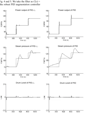
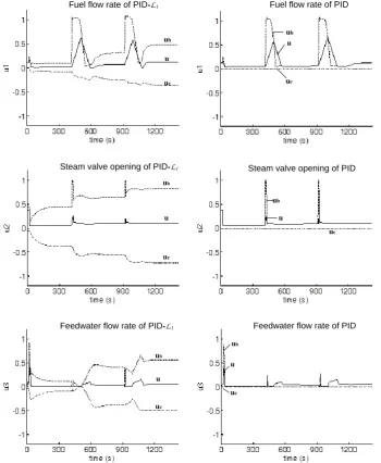
5.1. PID-L1 adaptive augmentation control system We make two wide-range load tracking operations and show the results in Fig. 6 for output variables and Fig. 7 for manipulated variables. For comparing each pair of the same variables in parallel, the output va-riables from the cascade robust PID-L1 augmentation adaptive control loops are shown on the left side in Fig. 6, and the output variables from the single robust PID controller loop are shown on the right side in Fig. 6. When the simulation time instant t=20s, let the boiler-turbine model change from the previous one into Eq. (28). The tracking results are shown in Fig. 6 and 7. From the output results in Fig. 6, we can see that the performance of the robust PID alone degrades greatly when large parameter variation of the plant arises. The PID-L1 augmentation controller shows good adaptivity to such unknown uncertainty as seen in the left-side sub figures in Fig. 6, due to the timely compensation by the signal ucfrom the
output of the L1 augmentation controller presented by the dash-dot curve shown in the left-side sub figures of Fig. 7. The signal uc of the robust PID-alone loop
keeps zero as seen in the right-side sub figures of Fig. 7 because the L1 augmentation controller is disconnected from the system. Therefore, the cascade PID-L1 augmentation controller works much better than the robust PID controller alone for the processes with unknown uncertainties. The L1 adaptive aug-mentation controller is very effective.
5.2. MPC-L1 adaptive augmentation control system
We design the OFL-MPC controller based on (21)-(26). The observer gain
L
is obtained by the pole placement for the augmented system (20). The placed poles are [0.09, 0.09, 0.12, 0.12, 0.135, -0.165]T. Other design parameters are chosen as Qt =
Fuel flow rate of PID-L1 Fuel flow rate of PID
u
uc uc
ub
ub
u
Steam valve opening of PID-L1 Steam valve opening of PID
uc
u
uc
u ub
ub
Feedwater flow rate of PID-L1 Feedwater flow rate of PID
u ub
ub
uc
u
uc
with Uncertainties
u=ub
uc=0
uc=0 u=ub
u=ub
uc=0
Figure 8. The results of the signle MPC loop without uncertainties
Left: output variables (solid line: output; dotted line: set-point); Right: manipulated variables
Rt = I3, Q = 0.5 I3, R = 150 I3, =40, ex=10, the
predictive horizon N=10, which is affordable on optimization computing time. Two simulation scenarios are made for the evaluation.
Case 1: The wide-range load tracking only by the MPC controller without uncertainty in the process. The results are shown in Fig. 8. This OFL-MPC we design has good robustness on the nonlinearity in a wide load range.
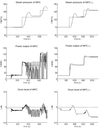
Case 2: The wide-range load tracking with varying of the model parameters as shown in Eq. (28) at the time instant t=120s. Fig. 9 shows the comparison on the output variables from the single MPC loop and the OFL-MPC-L1 augmentation loops. The sub figures on the left side in Fig. 9 show the output variables from the single Offset-free linear MPC loop. When the MPC controller works alone, it cannot deal with severe nonlinearity and unknown uncertainty. The system looks critical stable at both the medium and high load points. Whereas, the sub figures on the right
side in Fig. 9 show stable and good control performance of the OFL-MPC-L1 augmentation loops all the range. When the MPC controller and the L1
adaptive augmentation controller collaborate in the cascade loop, the obvious compensating control signals of the fuel flow rate, the steam valve and the feed-water flow rate are produced by the L1 adaptive augmentation controller, as shown in the right-side sub figures of Fig. 10. Each total control signal u = ub +uc s.t. (15) of u1, u2, u3 makes the closed-loop system
stable all the range. Fig. 10 shows the comparison on the manipulated variables from the single OFL-MPC loop and the OFL-MPC-L1 augmentation loops.
Steam pressure of MPC Steam pressure of MPC-L1
Power output of MPC Power output of MPC-L1
Drum level of MPC-L1
Drum level of MPC
Figure 9.Comparison on the output variables of single OFL-MPC loop (left) and OFL-MPC-L1 augmentation loops (right) in the
presence ofparameter variations(solid line: output; dotted line: set-point)
Remark 2. Both the robust PID controller and the OFL-MPC can work well in the nonlinear wide-range load tracking without uncertainties. Although the robust PID with AWBT function has better robustness than the OFL-MPC controller in terms of the unknown uncertainties in the simulations, both of their control qualities get much worse in this case. The simulations demonstrate that the L1 adaptive augmentation controller can effectively handle uncer-tainties including unmatched model, unmeasured dis-turbances and severe nonlinearity. This collaboration of the linear controllers and the L1 adaptive augmen-tation controller has much better adapaugmen-tation and robustness than the baseline controller alone for nonlinear systems.
We don’t change any parameter of the baseline controllers when the L1 adaptive augmentation con-troller is connected into the loops in the simulations
above. The low-pass filter of the L1 adaptive augmen-tation controller, which needs to ensure the L1 -gain condition [7], should be designed individually for different loops. Thus we have two different filters in the cascade PID-L1 adaptive augmentation controller and the MPC-L1 adaptive augmentation controller.
6. Conclusions
with Uncertainties
Fuel flow rate of MPC-L1
Fuel flow rate of MPC
uc
u ub
uc=0 u=ub
Steam Valve opening of MPC Steam Valve opening of MPC-L1
uc
u ub
uc=0 u=ub
Feedwater flow rate of MPC Feedwater flow rate of MPC-L1
uc
u ub
uc=0 u=ub
Figure10. Comparison on the manipulated variables of single MPC loop (left) and OFL-MPC-L1 augmentation loops (right) in
the presence ofparameter variations
approach is designed into the augmentation controller which takes effect and help with the linear controllers in the presence of uncertain conditions in the power-generation process. In this augmentation control scheme, the baseline controller, the L1 adaptive augmentation controller and the plant form a cascade control loop. A L1adaptive output feedback controller and the plant form into the inner-loop equivalent to a general plant with the desired dynamics for the outer baseline controllers to control. This fast-sampling L1
adaptive augmentation controller estimates the uncertainties and makes up their influence on the controlled process quickly. Because the transient tracking performance bound of the L1 adaptive controller can be rendered arbitrary small by reducing the step size of integration, the stability of the cascade control system can be ensured by tuning the sampling time of the inner L1 adaptive controller loop small enough. Two common controllers used in
power-generation process, the robust PID controller and offset-free linear MPC controller, are introduced and connected with the L1 adaptive augmentation controller in cascade. The simulation experiments on the boiler-turbine model with severe nonlinearity and time-varying parameters verify that the collaboration of the linear controllers and the L1 adaptive augmentation controller can greatly improve the closed-loop system stability under unknown uncertainties. Furthermore, it doesn’t need to change any parameter of the baseline controllers when a L1
promotion scheme for the control performance under unknown uncertainties in power plants.
Acknowledgments
This work was supported by the National Natural Science Foundation of China under Grant 51106024. The authors would like to express their appreciations to all the editors and reviewers for their precious time and work on this paper.
References
[1] K. R. Muske, T. A. Badgwell. Disturbance modeling for offset-free linear model predictive control. Journal of Process Control, 2002, Vol. 12, No. 5, 617-632. [2] U. Maeder, F. Borrelli, M. Morari. Linear offset-free
model predictive control. Automatica, 2009, Vol. 45, No. 10, 2214-2222.
[3] T. J. Zhang, G. Feng, X. J. Zeng. Output tracking of constrained nonlinear processes with offset-free input-to-state stable fuzzy predictive control. Automatica, 2009, Vol. 45, No. 4, 900-909.
[4] C. Cao, N. Hovakimyan. Design and analysis of a novel L1 adaptive control architecture with guaranteed
transient performance. IEEE Transactions on Automatic Control, 2008, Vol. 53, No. 4, 586-591. [5] C. Cao, N. Hovakimyan. L1 adaptive controller for a
class of systems with unknown nonlinearities: part I. In: Proceedings of the American control conference, ACC, Seattle, WA, United states, 2008, pp. 4093-4098. [6] C. Cao, N. Hovakimyan. L1 adaptive controller for
nonlinear systems in the presence of unmodelled dynamics: Part II. In: Proceedings of the American control conference, ACC, Seattle, WA, United states, 2008, pp. 4099-4104.
[7] C. Cao, N. Hovakimyan. Stability margins of L1
adaptive control architecture. IEEE Transactions on Automatic Control, 2010, Vol. 55, No. 2, 480-487. [8] N. Hovakimyan, C. Cao. L1 adaptive control theory:
guaranteed robustness with fast adaptation. SIAM, 2010.
[9] J. Luo, L. Pan, C. Cao. L1 adaptive controller for a nonlinear boiler-turbine system. In: Proceedings of the 53rd Annual ISA POWID Symposium, Summerlin, NV,
United states, 2010.
[10] C. Cao, N.Hovakimyan. L1 adaptive output-feedback
controller for non-strictly-positive-real reference systems: missile longitudinal autopilot design. Journal of Guidance, Control, and Dynamics, 2009, Vol. 32, 717-726.
[11] C. Cao, N. Hovakimyan. L1 adaptive output feedback
controller for systems of unknown dimension. IEEE Transactions on Automatic Control, 2008, Vol. 53, No. 3, 815-821.
[12] R. Bell, K. J. Åström. Dynamic models for boiler– turbine alternator units: data logs and parameter estimation for a 160MW unit. Technical Report, Department of Automatic Control, Lund Institute of Technology, Sweden, 1987.
[13] W. Tan, H. J. Marquez, T. Chen, J. Liu. Analysis and control of a nonlinear boiler-turbine unit. Journal of Process Control, 2005, Vol. 15, No. 8, 883-891. [14] P. Chen, J. Shamma. Gain-scheduled l1-optimal
control for boiler–turbine dynamics with actuator saturation. Journal of Process Control, 2004, Vol. 14, 263-277.
[15] U. C. Moon, K. Y. Lee. Step-response model development for dynamic matrix control of a drumtype boiler–turbine system. IEEE Transactions on Energy Conversion, 2009, Vol. 24, No. 2, 423-430.
[16] J. Wu, J. Shen, M. Krug, S. K. Nguang, Y. G. Li. GA-based nonlinear predictive switching control for a boiler-turbine system. Journal of Control Theory and Applications, 2012, Vol. 10, 100-106.
[17] M. Keshavarz, M. B. Yazdi, M. R. Jahed-Motlagh. Piecewise affine modeling and control of a boiler-turbine unit. Applied Thermal Engineering, 2010, Vol. 30, No. 8, 781-791.
[18] Y. G. Li, J. Shen, K. Y. Lee, X. C. Liu. Offset-free fuzzy model predictive control of a boiler-turbine system based on genetic algorithm. Simulation Modelling Practice and Theory, 2012, Vol. 26, 77-95.