Identification of Human Response to Virtual 3D Face Stimuli

(1)

Identification of Human Response to Virtual 3D Face Stimuli

Egidijus Vaškevičius

1

,

Aušra Vidugirienė

2

, Vytautas Kaminskas

3

Department of Systems’ Analysis, Vytautas Magnus University Vileikos st. 8, LT – 44404, Kaunas Lithuania

e-mail: [email protected], [email protected], 3_{[email protected]}

http://dx.doi.org/10.5755/j01.itc.43.1.5927

Abstract. This paper introduces identification results of human response to virtual 3D face stimuli. Observations of human reactions are done using preprocessed EEG (electroencephalogram) signals: excitement, meditation, frustration, engagement/boredom. Virtual 3D face features – distance between eyes, nose width, and chin width – are used as stimuli. Cross-correlation analysis demonstrated that dynamical relations between human reactions and stimuli exist. Input-output models describing relations between stimuli and corresponding human reactions are built. A new input-output model building method is proposed that allows building stable models with the least output prediction error. Models’ validation results demonstrate relatively high prediction accuracy of human reactions.

Keywords: 3D face stimuli; human reaction; cross-correlation analysis; input-output model; model parameter estimation; model validation.

1. Introduction

Virtual environments are becoming a part of our daily life including computer games, work tasks, various mental and physical training programs, e-learning, online shopping, and specialized software. These environments affect the users in different extents and ways. The influence can be both positive and negative. Various studies introduce investigations, where human state observation is an important task. Several of them concentrates on stress evaluation and training when using virtual environments for military purposes and curing post-traumatic stress disorder [15]. Other focuse on neuro-marketing [11], [12], adaptive virtual mediator services [14], social networks [22], and learning applications [1], [4].

In order to protect people from various harmful effects to their health (e.g. stress) that virtual environment can cause [17], to create training applications, or to implement/use virtual mediator services [7], control mechanisms of virtual environment object features and the interactions have to be modeled [5], [10].

The most effective way to observe a state of a person in a real time is to monitor human bio-signals [19]. A variety of human bio-signals such as galvanic skin response, pulse, magnetoencephalography (MEG), heart rate, EEG, etc. are used for this purpose and plenty of methods and techniques help to

measure and analyze the signals [23]. We have chosen to use EEG-based signals for human affective state monitoring because of the reliability and quick response [18], [6].

In this research, a virtual 3D face was used as a stimulus for eliciting human reaction. It is known that the majority of information to another person when communicating is transferred by face features [13]. A person is used to react to the smallest face feature changes during a very short time [21]. We have created and used a realistic virtual 3D face model. Human reactions when he/she is observing visual stimuli (3D face changes) were investigated.

Our previous investigations on the dependencies between virtual stimuli and human affective responses demonstrated that in certain circumstances the dependencies exist and there is a need of further research [20].

(2)

2. Observations and data

Features of virtual 3D face (distance between eyes, nose width, and chin width) were used for input and EEG-based human reaction signals (excitement, meditation, frustration, engagement/boredom) of a person were measured as output (Fig. 1). These output signals were chosen as important features in learning, and stress regulation. The output signals were recorded using Emotive Epoc device.The device records EEG inputs from 14 channels (according to international 10-20 locations): AF3, F7, F3, FC5, T7, P7, O1, O2, P8, T8, FC6, F4, F8, AF4 [3].

Figure 1. Input-Output scheme for the experiments

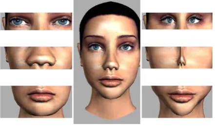
Seven 3D woman faces were created using Autodesk MAYA. One 3D woman face was used as a “neutral” one (Fig. 2, middle). The other faces were formed by changing face features in an extreme manner: large and small distance between eyes (Fig. 2, left and right, top), wide and thin nose (Fig. 2, left and right, middle), wide and thin chin (Fig. 2, left and right, bottom). After importing the 3D faces into Unity 3D engine, the transitions between the same kind of features in the face were programmed using morph target’s method.

Figure 2. A “neutral” 3D woman face (middle) and limit cases of features: the largest (left top) and the smallest (right

top) distance between eyes, the widest (left middle) and the thinnest (right middle) nose, the widest (left bottom) and the

thinnest (right bottom) chin

There were two types of input signals used. TYPE 1 input signals (Fig. 3, top) were formed when neutral face was equal to 0, the largest (widest) feature was equal to 1.8 and the smallest (thinnest) feature was equal to -1.8. The values in-between were changed linearly. Time interval between

largest/smallest value and zero (normal face) was 10 s. The features were changing continuously: from normal to extremely wide, then back to normal and to extremely thin, then again to normal and to extremely wide and again back to normal. The animated tests were prepared for every of three features: distance between eyes, nose width and chin width.

Figure 3. TYPE 1 and TYPE 2 input signals: values variation of corresponding face feature modifications TYPE 2 input signals (Fig. 3, bottom) were formed when changing the 3D face features suddenly. “Small distance-between-eyes”, “thin nose” or “thin chin” was shown for some period of time, then the picture was suddenly changed to “normal” and after some time to “large distance-between-eyes”, “wide nose” or “wide chin” and again to “normal”. It was repeated two times with different time steps between each change. “Neutral” face was equal to 0, “largest dis-tance-between-eyes”, “widest nose” or “widest chin” were equal to 1.25 and the smallest features – to -1.25.

Output signals – excitement, meditation, frustration and engagement/boredom – varied from 0 to 1. If excitement, meditation, frustration and engage-ment were low, the value was 0 or close to 0 and if they were high, the values of parameters were 1 or close to 1. The signals were recorded with the sampling period of T0=0.5 s.

Five volunteers (volunteers no. 1-3 were female, and volunteers no. 4-5 were male) were tested. A volunteer was watching three animated scenes of approximately 1 minute one after another, and EEG-based signals were measured simultaneously using Emotiv Epoc device. The recorded preprocessed signals were stored for later analysis.

3. Correlation analysis

To estimate the possible relations between virtual stimuli and human reaction signals, a cross-correlation analysis between stimuli (3D virtual face features) and response (EEG-based reaction) signals was performed.

Cross-covariation functions between input and output signals and auto-covariation functions of input and output signals are used for this purpose [16]:

0 10 20 30 40 50 -2

0 2

time, s TYPE 2

0 10 20 30 40 50 -2

0 2

(3)

𝑅𝑦𝑥[𝜏] =_{𝑁 �}1 (𝑦𝑡− 𝑦�)(𝑥𝑡+𝜏− 𝑥̅) 𝑁−𝜏

𝑡=1

𝑅𝑥𝑥[𝜏] =_{𝑁 �}1 (𝑥𝑡− 𝑥̅)(𝑥𝑡+𝜏− 𝑥̅) 𝑁−𝜏

𝑡=1

𝑅𝑦𝑦[𝜏] =_{𝑁 �}1 (𝑦𝑡− 𝑦�)(𝑦𝑡+𝜏− 𝑦�) 𝑁−𝜏

𝑡=1

(1)

where

𝑥̅=_{𝑁 � 𝑥}1 𝑡 𝑁

𝑡=1

, 𝑦�=_{𝑁 � 𝑦}1 𝑡 𝑁

𝑡=1

(2)

are the averages of input and output, τ= 0, ±1, … and N=115.

Cross-correlation functions between both types of input signals (TYPE 1 and TYPE 2) and all output sig-nals for volunteer no. 1 are demonstrated in Figs. 4−6.

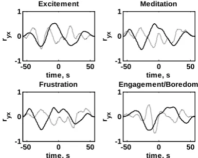
Figure 4. Cross-correlation functions between distance between eyes input feature and all output features for

volunteer no.1. Solid line denotes input Type 1, dotted line denotes input Type 2

Figure 5. Cross-correlation functions between nose width input feature and all output features for volunteer no.1. Solid

line denotes input Type 1, dotted line denotes input Type 2

Figure 6. Cross-correlation functions between chin width input feature and all output features for volunteer

no.1. Solid line denotes input Type 1, dotted line denotes input Type 2

Maximum cross-correlation function values

max

𝜏 �𝑟𝑦𝑥[0]�= max𝜏 �

𝑅𝑦𝑥[𝜏] �𝑅𝑦𝑦[0]𝑅𝑥𝑥[0]�

(3)

were estimated for each stimulus and the corresponding response signal pair. The estimates of the maximum cross-correlation function values are shown in Table 1 and Table 2.

Table 1. Maximum cross-correlation function values when Type 1 input signal is used

V

o

lu

n

teer n

o

.

Input (stimulus)

Output (reaction)

E

xci

tem

en

t

M

ed

it

a

tio

n

F

ru

st

ra

ti

o

n

E

ng

age

m

ent

/

B

or

edom

1

Distance between eyes 0.55 0.75 0.88 0.81

Nose width 0.51 0.55 0.53 0.55

Chin width 0.73 0.57 0.59 0.63

2

Nose width 0.73 0.51 0.47 0.66

Chin width 0.35 0.75 0.43 0.37

3

Nose width 0.30 0.67 0.80 0.62

Chin width 0.38 0.74 0.43 0.38

4

Nose width 0.47 0.65 0.59 0.66

Chin width 0.40 0.64 0.43 0.55

5

Nose width 0.71 0.68 0.75 0.82

Chin width 0.70 0.66 0.54 0.62

The shift of the maximal values of cross-correlation functions in relation to 𝑟_𝑦𝑥 [0] allow stating that there exist dynamic relations between virtual

-50 0 50 -1

0 1

Excitement

time, s

r yx

-50 0 50 -1

0 1

Meditation

time, s

r yx

-50 0 50 -1

0 1

Frustration

time, s

r yx

-50 0 50 -1

0 1

Engagement/Boredom

time, s

r yx

-50 0 50 -1

0 1

Excitement

time, s

r yx

-50 0 50 -1

0 1

Meditation

time, s

r yx

-50 0 50 -1

0 1

Frustration

time, s

r yx

-50 0 50 -1

0 1

time, s

r yx

-50 0 50 -1

0 1

Excitement

time, s

r yx

-50 0 50 -1

0 1

Meditation

time, s

r yx

-50 0 50 -1

0 1

Frustration

time, s

r yx

-50 0 50 -1

0 1

time, s

(4)

stimuli and human reactions to them. High cross-correlation values justify a possibility to use linear dynamic models.

Table 2. Maximum cross-correlation function values when Type 2 input signal is used

V

o

lu

n

teer n

o

.

Input (stimulus)

Output (reaction)

E

xci

tem

en

t

M

ed

it

a

tio

n

F

ru

st

ra

ti

o

n

E

ng

age

m

ent

/

B

or

edom

1

Nose width 0.54 0.47 0.45 0.68

Chin width 0.53 0.56 0.47 0.38

2

Nose width 0.49 0.41 0.43 0.61

Chin width 0.63 0.56 0.57 0.38

3

Nose width 0.47 0.49 0.47 0.68

Chin width 0.55 0.40 0.42 0.57

4

Nose width 0.50 0.44 0.46 0.41

Chin width 0.53 0.63 0.64 0.54

5

Nose width 0.43 0.50 0.45 0.52

Chin width 0.46 0.56 0.36 0.48

4. Mathematical model building

All dependencies between virtual object stimuli and human reactions are described by input-output structure models [8]:

𝐴(𝑧−1₎_𝑦

𝑡=𝐵(𝑧−1)𝑥𝑡+𝜀𝑡 (4)

𝐵(𝑧−1_{) =}_{� 𝑏} 𝑗𝑧−𝑗, 𝑚

𝑗=0

𝐴(𝑧−1_{) = 1 +}_{� 𝑎} 𝑖𝑧−𝑖 𝑛

𝑖=1

(5)

where 𝑦_𝑡 is an output (excitement, engagement/ boredom meditation, frustration or) and 𝑥_𝑡 is an input (distance between eyes, nose width, chin width) signals respectively calculated as

𝑦𝑡=𝑦(𝑡𝑇0), 𝑥𝑡=𝑥(𝑡𝑇0) (6) with sampling period 𝑇₀, 𝜀_𝑡 corresponds to noise signal and z-1 is the backward-shift operator (z−1x_t=

xt−1).

Eq. (4) can be expressed in the following form:

𝑦𝑡=� 𝑏𝑗𝑥𝑡−𝑗 𝑚

𝑗=0

− � 𝑎𝑖𝑦𝑡−𝑖 𝑛

𝑖=1

+𝜀𝑡 . (7)

Model parameters (coefficients of the polynomials (5)) and model order (degrees m and n of polynomials (5)) are unknown. They have to be estimated

according to the observations obtained during the experiments with the volunteers.

It is not difficult to show that in the case of using the model, the following relationship exists between covariation functions:

𝑅𝑦𝑥[𝜏] =� 𝑏𝑗 𝑚

𝑗=0

𝑅𝑥𝑥[𝜏 − 𝑗]− � 𝑎𝑖 𝑛

𝑖=1

𝑅𝑦𝑥[𝜏 − 𝑖] .(8)

Equation (8) can be expressed as a linear regression equation:

𝑅𝑦𝑥[𝜏] =𝜷𝜏𝑇𝒄 (9)

where

𝜷𝜏𝑇 = [ 𝑅𝑥𝑥[𝜏],𝑅𝑥𝑥[𝜏 −1], … ,𝑅𝑥𝑥[𝜏 − 𝑚], −𝑅𝑦𝑥[𝜏 −1], … ,−𝑅𝑦𝑥[𝜏 − 𝑛] ]

(10)

𝒄𝑇 ₌_�𝑏

0,𝑏1, … ,𝑏𝑚,𝑎1,𝑎2, … ,𝑎𝑛� (11) and T is a vector transpose sign.

For the estimation of unknown parameter vector c

we use a method of least squares [8]:

𝒄�=𝑸−1_𝒒 ₍₁₂₎

𝑸=�𝑀_𝜏=−𝑀𝜷𝜏𝜷𝜏𝑇, 𝒒=�𝑀_𝜏=−𝑀𝑅𝑦𝑥[𝜏]𝜷𝜏 (13)

where M is the number of covariation function values used.

Model parameter estimates’ vector 𝒄� is calculated when M=0, 1, … and model stability condition is verified [8]. It means that the following polynomial

𝐴̂𝑀(𝑧) =𝑧𝑛𝐴̂𝑀(𝑧−1) =𝑧𝑛+� 𝑎�𝑖𝑧𝑛−𝑖 𝑛

𝑖=1

(14)

roots

𝑧𝑖𝐴: 𝐴̂𝑀(𝑧) = 0,𝑖= 1, 2, … ,𝑛 (15) have to be in the unit disk

�𝑧𝑖𝐴� ≤1 (16)

In that way, we get a subset 𝛺_𝑀 with M values where the models are stable. From this subset we choose

𝑀�: 𝑚𝑖𝑛{𝜎𝜀[𝑀|𝑚,𝑛], 𝑀𝑀𝛺𝑀} (17) where

𝜎𝜀[𝑀|𝑚,𝑛] =�_{𝑁 � 𝜀̂}1 𝑡2[𝑀|𝑚,𝑛] 𝑁

𝑡=1

(18)

(5)

𝑦�𝑡|𝑡−1[𝑀|𝑚,𝑛] =

=𝑧�1− 𝐴̂𝑀(𝑧−1)�𝑦𝑡−1+𝐵�𝑀(𝑧−1)𝑥𝑡

(20)

is one step output prediction [9] and z is the forward-shift operator (zy_t= y_t+1).

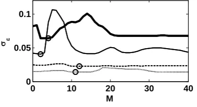
Figs. 7-8 demonstrate examples of prediction error standard deviations with every M value for each output signal (when the same input signal is used).

Figure 7. Prediction error standard deviation, nose width input (Type 2), volunteer no. 4, model order m=1, n=1.

Lines: solid thick– excitement, dotted– meditation, solid thin– frustration, dashed– engagement/boredom

Figure 8. Prediction error standard deviation, distance-between-eyes input (Type 2), volunteer no. 1, model order m=0, n=2. Lines: solid thick– excitement,

dotted– meditation, solid thin– frustration, dashed– engagement/boredom

The circles indicate M values where the error standard deviations were the smallest in each output case. If models are not stable with certain M values, the error standard deviations are not estimated and there are discontinuities in the error standard deviations signal.

Estimates of the model orders – 𝑚� and 𝑛� – are defined from the following conditions:

𝑛�: �𝜎𝜀�𝑀�|𝑚,𝑛+ 1� − 𝜎𝜀�𝑀�|𝑚,𝑛� 𝜎𝜀�𝑀�|𝑚,𝑛� � ≤ 𝛿,

𝑛= 1,2, …

𝑚�: �𝜎𝜀�𝑀�|𝑚+ 1,𝑛� − 𝜎𝜀�𝑀�|𝑚,𝑛� 𝜎𝜀�𝑀�|𝑚,𝑛� � ≤ 𝛿,

𝑚= 0,1, … ,𝑛

(21)

where 𝛿> 0 is a chosen constant value. Usually in the practice of identification 𝛿 ∈[0,001 ÷ 0,01] what

corresponds to a relative variation of prediction error standard deviation from 0,1% to 1%.

This way a stable input-output model is built that ensures the best one step output signal prediction.

Figs. 9-10 demonstrate prediction error standard deviations for an input-output pair when n=1, 2 and m=0, 1, 2 for each model. Fig. 9. shows error standard deviation when distance-between-eyes input (Type 1) and engagement/boredom output is used for prediction for every of five models. Fig. 10. shows the same with chin width input (Type 2) and excitement output signal.

Figure 9. Prediction error standard deviation, volunteer no. 2, distance-between-eyes input signal (Type 1),

engagement/boredom output signal

Figure 10. Prediction error standard deviation, volunteer no. 3, chin width input signal (Type 2),

excitement output signal

5. Models validation

Every stimuli type requires 12 input-output models for each volunteer. Each model is selected from five possible models (when n=1, 2; m=0, …, n) using the rule (21). Two types of stimuli for each of five volunteers were used, so 120 models were analyzed. The analysis of five volunteers’ data showed that relations between each of three stimuli (distance between eyes, nose width, and chin width) and excitement output signal can be modeled when model order is 𝑚�= 0 and 𝑛�= 1. Relations between each of three stimuli and meditation, frustration and engagement/boredom output signals are best modeled when model order is 𝑚�= 0 and 𝑛�= 2.

Every model was validated through the output signal (excitement, meditation, engagement/boredom, frustration) prediction analysis. The predicted output signals have the following expression [8]:

0 10 20 30 40

0 0.05 0.1

σ ε

M

0 10 20 30 40

0 0.05 0.1

σ ε

(6)

𝑦�𝑡+1|𝑡=𝑧�1− 𝐴̂(𝑧−1)�𝑦𝑡+𝐵�(𝑧−1)𝑥𝑡+1=

=− � 𝑎�𝑖𝑦𝑡+1−𝑖+ 𝑛�

𝑖=1

� 𝑏�𝑗𝑥𝑡+1−𝑗 𝑚�

𝑗=0

(22)

Prediction accuracies were evaluated using the following measures:

• prediction error standard deviation

𝜎𝜀=�_𝑁1� �𝑦𝑡+1− 𝑦�𝑡+1|𝑡�2 𝑁−1

𝑡=0 (23)

• relative prediction error standard deviation

𝜎�𝜀=�_𝑁1� �𝑦𝑡+1_𝑦−𝑦�_𝑡+1𝑡+1|𝑡� 2 𝑁−1

𝑡=0

∗100% (24)

• and average absolute relative prediction error

|𝜀̅| =1_𝑁� �𝑦𝑡+1−𝑦�𝑡+1|𝑡

𝑦𝑡+1 �

𝑁−1

𝑡=0 ∗100% (25)

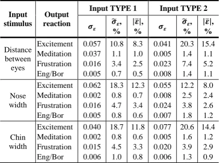
Measures of prediction accuracy (23) - (25) are given in Tables 3-7.

Table 3. Prediction accuracy measures, volunteer no. 1

Input stimulus

Output reaction

Input TYPE 1 Input TYPE 2

𝝈𝜺 𝝈�_%𝜺, |_%𝜺�|, 𝝈𝜺 𝝈�_%𝜺, |_%𝜺�|, Distance between eyes Excitement Meditation Frustration Eng/Bor 0.044 0.006 0.011 0.010 11.5 1.9 2.1 1.6 7.79 1.5 1.4 1.5 0.054 0.010 0.023 0.010 13.8 3.0 4.0 1.7 8.6 2.6 2.8 1.7 Nose width Excitement Meditation Frustration Eng/Bor 0.038 0.005 0.017 0.003 16.0 2.0 4.9 0.6 10.5 1.4 3.3 0.5 0.031 0.007 0.019 0.013 16.1 2.2 7.4 2.4 9.4 1.7 5.0 2.2 Chin width Excitement Meditation Frustration Eng/Bor 0.026 0.007 0.017 0.004 10.9 2.7 4.1 0.8 7.0 1.7 2.9 0.5 0.017 0.005 0.016 0.014 8.2 2.6 4.8 2.9 5.2 1.7 3.6 2.8

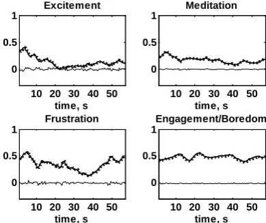
Figs. 11-22 demonstrate observed output signals, their predictions and prediction errors.

(7)

Figure 11. Volunteer no. 1 (female), distance between eyes TYPE 1 input. Solid thick line – observed signal, dotted

line – predicted signal, solid thin line – prediction error between observed and predicted signal

Figure 12. Volunteer no. 1 (female), nose width TYPE 1 input. Solid thick line – observed signal, dotted line – predicted signal, solid thin line – prediction

error between observed and predicted signal

Figure 13. Volunteer no. 1 (female), chin width TYPE 1 input. Solid thick line – observed signal, dotted line – predicted signal, solid thin line – prediction

Figure 14. Volunteer no. 1 (female), distance between eyes TYPE 2 input. Solid thick line – observed signal, dotted

Figure 15. Volunteer no. 1 (female), nose width TYPE 2 input. Solid thick line – observed signal, dotted line – predicted signal, solid thin line – prediction

Figure 16. Volunteer no. 1 (female), chin width TYPE 2 input. Solid thick line – observed signal, dotted line – predicted signal, solid thin line – prediction

10 20 30 40 50 0

0.5 1

Excitement

time, s

10 20 30 40 50 0

0.5 1

Meditation

time, s

10 20 30 40 50 0

0.5 1

Frustration

time, s

10 20 30 40 50 0

0.5 1

time, s

10 20 30 40 50 0

0.5 1

Excitement

time, s

10 20 30 40 50 0

0.5 1

Meditation

time, s

10 20 30 40 50 0

0.5 1

Frustration

time, s

10 20 30 40 50 0

0.5 1

time, s

10 20 30 40 50 0

0.5 1

Excitement

time, s

10 20 30 40 50 0

0.5 1

Meditation

time, s

10 20 30 40 50 0

0.5 1

Frustration

time, s

10 20 30 40 50 0

0.5 1

time, s

10 20 30 40 50 0

0.5

1 Excitement

time, s

10 20 30 40 50 0

0.5

1 Meditation

time, s

10 20 30 40 50 0

0.5 1

Frustration

time, s

10 20 30 40 50 0

0.5 1

time, s

10 20 30 40 50 0

0.5 1

Excitement

time, s

10 20 30 40 50 0

0.5 1

Meditation

time, s

10 20 30 40 50 0

0.5 1

Frustration

time, s

10 20 30 40 50 0

0.5 1

time, s

10 20 30 40 50 0

0.5 1

Excitement

time, s

10 20 30 40 50 0

0.5 1

Meditation

time, s

10 20 30 40 50 0

0.5 1

Frustration

time, s

10 20 30 40 50 0

0.5 1

(8)

Figure 17. Volunteer no. 4 (male), distance between eyes TYPE 1 input. Solid thick line – observed signal, dotted

Figure 18. Volunteer no. 4, (male) nose width TYPE 1 input. Solid thick line – observed signal, dotted line – predicted signal, solid thin line – prediction

Figure 19. Volunteer no. 4 (male), chin width TYPE 1 input. Solid thick line – observed signal, dotted line – predicted signal, solid thin line – prediction

Figure 20. Volunteer no. 4 (male), distance between eyes TYPE 2 input. Solid thick line – observed signal, dotted

Figure 21. Volunteer no. 4 (male), nose width TYPE 2 input. Solid thick line – observed signal, dotted line – predicted signal, solid thin line – prediction

Figure 22. Volunteer no. 4(male), chin width TYPE 2 input. Solid thick line – observed signal, dotted line – predicted

signal, solid thin line – prediction error between observed and predicted signal

10 20 30 40 50 0

0.5 1

Excitement

time, s

10 20 30 40 50 0

0.5 1

Meditation

time, s

10 20 30 40 50 0

0.5 1

Frustration

time, s

10 20 30 40 50 0

0.5 1

time, s

10 20 30 40 50 0

0.5 1

Excitement

time, s

10 20 30 40 50 0

0.5 1

Meditation

time, s

10 20 30 40 50 0

0.5 1

Frustration

time, s

10 20 30 40 50 0

0.5 1

time, s

10 20 30 40 50 0

0.5 1

Excitement

time, s

10 20 30 40 50 0

0.5 1

Meditation

time, s

10 20 30 40 50 0

0.5 1

Frustration

time, s

10 20 30 40 50 0

0.5 1

time, s

10 20 30 40 50 0

0.5 1

Excitement

time, s

10 20 30 40 50 0

0.5 1

Meditation

time, s

10 20 30 40 50 0

0.5 1

Frustration

time, s

10 20 30 40 50 0

0.5 1

time, s

10 20 30 40 50 0

0.5 1

Excitement

time, s

10 20 30 40 50 0

0.5 1

Meditation

time, s

10 20 30 40 50 0

0.5 1

Frustration

time, s

10 20 30 40 50 0

0.5 1

time, s

10 20 30 40 50 0

0.5 1

Excitement

time, s

10 20 30 40 50 0

0.5 1

Meditation

time, s

10 20 30 40 50 0

0.5 1

Frustration

time, s

10 20 30 40 50 0

0.5 1

(9)

Results of model validation demonstrate that average absolute relative prediction errors of meditation and engagement/boredom signals in all five volunteer cases were less than 1.5 %, frustration – less than 3.5 %, and excitement – less than 10 %. The corresponding relative error standard deviation averages are less than 2 % for meditation and engagement/boredom, less than 4.5 % for frustration and less than 15 % for excitement output signals.

Predictive models are necessary in the design of predictor-based self-tuning control systems [2], [9]. High prediction accuracies of the built models allow expecting that they can be a basis for this type control systems of human reactions to virtual stimuli. Such systems could serve as a mean for regulation of human attention level in learning applications as well as in computerized workplaces for dispatchers.

6. Conclusions

Cross-correlation analysis demonstrated that there is a relatively high correlation between stimuli (input) and human response (output) and that evidences the existence of linear dynamic relations between them.

When using cross- and auto-correlation functions, a new method for building an input-output modelwas proposed. It allows building a stable model for output signal prediction with the least prediction error. The models allow describing the dynamic dependencies between virtual 3D face that changes during time and the reactions to it.

Validation results of the models demonstrate that every volunteer reacted to the stimuli individually and the reactions are described by input-output models with different estimates of polynomial coefficient.

The models describe the dependencies between every input signal (distance between eyes, nose width and chin width) and every corresponding output signal (excitement, meditation, engagement/boredom, and frustration) in high accuracy: averages of absolute relative prediction errors of engagement/boredom and meditation signals in five volunteer cases were less than 1.5 %, frustration – less than 3.5 %, and excitement – less than 10 %.

Acknowledgments

Postdoctoral fellowship of Ausra Vidugiriene is funded by European Union Structural Funds project ”Postdoctoral Fellowship Implementation in Lithuania” within the framework of the Measure for Enhancing Mobility of Scholars and Other Researchers and the Promotion of Student Research (VP1-3.1-ŠMM-01) of the Program of Human Resources Development Action Plan.

References

[1] R. Ciceri, S. Balzarotti. From Signals to Emotions: Applying Emotion Models to HM Affective

Interactions. In: Affective Computing: Emotion

Modeling, Synthesis and Recognition, ITech,

Education and Publishing, 2008, pp. 271-296. Available at: http://dx.doi.org/10.5772/6176.

[2] D. W. Clarke. Advances in Model Predictive Control. Oxford Science Publications, UK, 1994.

[3] Emotiv Epoc specifications. Brain-computer interface technology. Available at: http://www.emotiv.com/ upload/manual/sdk/EPOCSpecifications.pdf.

[4] S. Fatahi, N. Ghasem-Aghaee. An Effective Intelligent Educational Model Using Agent with Personality and Emotional Filters. In: Proceedings of the World Congress on Engineering, Vol. 1, 2010, pp. 142-147. Available at: http://www.iaeng.org/ publication/WCE2010/WCE2010_pp142-147.pdf. [5] J. Hoey, T. Schroeder, A. Alhothali. Bayesian Affect

Control Theory. In: IEEE 2013 Humaine Association Conference on Affective Computing and Intelligent Interaction, Geneva, Switzerland, 2013, pp. 166-172. Available at: http://dx.doi.org/10.1109/ACII.2013.34. [6] C. Hondrou, G. Caridakis. Affective, Natural

Interaction Using EEG: Sensors, Application and Future Directions. In: Artificial Intelligence: Theories and Applications. LNCS Vol. 7297, Springer-Verlag Berlin Heidelberg, 2012, pp. 331-338. Available at: http://dx.doi.org/10.1007/978-3-642-30448-4_42. [7] M. E. Hoque, M. Courgeon, J.-C. Martin, B. Mutlu,

R. W. Picard. MACH: My Automated Conversation coacH. In: 15th International Conference on

Ubiquitous Computing (Ubicomp), Zurich,

Switzerland, September, 2013, pp. 697-706. Available at: http://dx.doi.org/10.1145/2493432.2493502. [8] V. Kaminskas. Dynamic Systems Identification via

Discrete-Time Observations, Part1 – Statistical Method Foundations. Estimation in Linear Systems, Vilnius: Mokslas, 1982, (in Russian).

[9] V. Kaminskas. Predictor-based self tuning control with constraints. Model and Algorithms for Global Optimization, Optimization and Its Applications, Vol. 4, Springer, 2007, pp. 333-341. Available at: http://dx.doi.org/10.1007/978-0-387-36721-7_20. [10] R. N. Khushaba, L. Greenacre, S. Kodagoda,

J. Louviere, S. Burke, G. Dissanayake. Choice modeling and the brain: A study on the Electroencephalogram (EEG) of preferences. Expert Systems with Applications, Vol. 39, Is. 16, 2012, pp. 12378–12388. Available at: http://dx.doi.org/10. 1016/j.eswa.2012.04.084.

[11] R. N. Khushaba, Ch. Wise, S. Kodagoda, J. Louviere, B. E. Kahn, C. Townsend. Consumer neuroscience: Assessing the brain response to marketing stimuli using electroencephalogram (EEG) and eye tracking. Expert Systems with Applications, Vol. 40, Is. 9, pp. 3803-3812. Available at http://dx.doi.org/10.1016/j.eswa.2012.12.095.

[12] Y. Liu, O. Sourina, M. Rizqi Hafiyyandi. EEG-based Emotion-adaptive Advertising. In: IEEE 2013 Humaine Association Conference on Affective

Computing and Intelligent Interaction, Geneva,

Switzerland, 2013, pp. 843-848. Available at: http://dx.doi.org/10.1109/ ACII.2013.158.

[13] A. Mehrabian. Silent messages: Implicit communication of emotions and attitudes. Belmont, CA: Wadsworth Publishing Company, 1981.

(10)

Psycho-physiological Measures for the Design and Behavior of Socially-Aware Avatars in Ubicomp Environments. In: CHI 2010, April, Atlanta, GA, USA pp. 1-4.

[15] A. Rizzo, J. G. Buckwalter, B. John, B. Newman, T. Parsons, P. Kenny, J. Williams. STRIVE: Stress Resilience In Virtual Environments: A Pre-Deployment VR System for Training Emotional Coping Skills and Assessing Chronic and Acute Stress Responses. In: Medicine Meets Virtual Reality 19, IOS Press, 2012, pp. 379-385. Available at: http://dx.doi.org/10.3233/978-1-61499-022-2-379. [16] J. G. Proakis, D. G. Manolakis. Digital signal

Processing: Principles, Algorithms, and Application, 4th edition, Pearson Prentice Hall, 2007.

[17] A. Sano, R. W. Picard. Stress recognition using wearable sensors and mobile phones. In: IEEE 2013 Humaine Association Conference on Affective

Computing and Intelligent Interaction, Geneva,

Switzerland, 2013, pp. 671-676. Available at: http://dx.doi.org/10.1109/ ACII.2013.117.

[18] O. Sourina, Y. Liu. A Fractal-based Algorithm of Emotion Recognition from EEG using Arousal-valence model. In: Proc. Biosignals, Rome,2011, pp. 209-214. [19] Suprijanto, L. Sari, V. Nadhira, IGN. Merthayasa,

I. M. Farida. Development System for Emotion

Detection Based on Brain Signals and Facial Images.

In: World Academy of Science, Engineering and

Technology 26, 2009, pp. 931-938. Available at:

http://waset.org/ publications/8769.

[20] E. Vaskevicius, A. Vidugiriene, V. Kaminskas. Investigation of dependencies between virtual 3d face stimuli and emotion-based human responses. In: Proc. of the 8th International Conference on Electrical and Control Technologies, Kaunas, 2013, pp. 64-69. [21] J. Willis, A. Todorov. First Impressions: Making Up

Your Mind After a 100-Ms Exposure to a Face. In: Psychological science, Vol. 17, No. 7, 2006,

pp. 592−598. Available at:

http://dx.doi.org/10.1111/j.1467-9280.2006. 01750.x. [22] Y. Zhang, J. Tang, J. Sun, Y. Chen, J. Rao.

MoodCast: Emotion Prediction via Dynamic Continuous Factor Graph Model. In: IEEE 10th International Conference on Data Mining, Sydney,

2010, pp. 1193-1198. Available at:

http://dx.doi.org/10.1109/ICDM.2010.105.