Adaptive Sensing Using Data Prediction for Wireless Sensor Networks

Adaptive Sensing Using Data Prediction for Wireless

Sensor Networks

Vipan Arora

Research Scholar, NIT, Hamirpur (H.P.) Associate Professor, NIT, Hamirpur (H.P.)

Dr. T.P. Sharma

Date of publication (dd/mm/yyyy): 30/04/2017

Abstract – Wireless sensor networks are generally deployed in inaccessible terrains for monitoring certain physical parameters like temperature, humidity, radiations, vibrations etc. As large numbers of sensor nodes are sensing the region, it is likely that sensed data may be both spatially and temporally correlated. These correlations can be exploited to reduce communication cost by reducing data exchange by setting sampling rate of sensor nodes appropriately. In this paper, we propose an Adaptive Sensing Using Data Prediction (ASDP) scheme that controls the sensing rates of sensor nodes. To do this, scheme utilizes the local estimation at every cluster head and finds correlation among different values at cluster head level. The strategy thrives at dynamically altering the sensing frequency of sensor nodes based on this correlation. Highly correlated values depict the static nature of the event under observations whereas highly uncorrelated values points towards very dynamic event. Thus, by dynamically setting the sensing frequency, generation of redundant data in case of static event can be minimized. Also, missing some important readings due to low sensing frequency can also be taken care of. Simulation results show that ASDP provides substantial energy saving as compared to other adaptive sensing schemes.

Keywords – Wireless Sensor Networks, Sensor Node, Adaptive Sensing, Sensing Rate, Energy Efficient.

I.

I

Wireless Sensor Network (WSN) consists of large number of sensor nodes (SNs) which are small in size, low cost and have limited memory, sensing, computation and wireless communication capabilities. SNs measure the ambient conditions from the environment surrounding them. In these applications, SNs are deployed to operate autonomously in unattended environments. In addition to the ability to probe its surroundings, each sensor has an on board radio to be used for sending the collected data to a base-station either directly or over a multi-hop path [1][2].

SNs are energy constrained devices. Energy consumption is generally associated with communication and more the communication more is the energy consumption. The solution to this problem could be the periodic replacement of the node battery. But, this is not viable every time as SNs may be inaccessible in some applications such as monitoring snow avalanches, tsunami or volcanoes etc. Further, different applications may require persistent long-term data collection because the gathered data make sense only if the data collection procedure lasts for months or even years without interruption. Therefore, data collection strategy must be carefully designed to reduce energy consumption at SNs, so as to prolong the network lifetime. [3] [4].

In sensor networks, sending large amount of raw data directly to the sink can lead to several undesirable problems. First, the quality of data may be deteriorated by packets losses due to the limited bandwidth of SNs. Second, intensive data collection incurs excessive communication traffic and potentially results in network congestions. Also, excessive communication results in the exhaustion of SNs batteries. Third, intensive data collection leads to excessive energy consumption during sensing. Authors in [5][6] report that the lifetime of a sensor network can be increased from one month to more than eighteen months by lowering the data flow rates of SNs.

As larger numbers of SNs are deployed for sensing data, the sensing process is likely to produce huge amount of redundant or correlated data. The nearby SNs tend to collect similar data. To increase the life time of network, the energy consumption of SNs must be reduced. To achieve this, spatial or temporal correlations can be exploited to manage the set of nodes that collect redundant data. For efficient data gathering with a minimum use of limited resources, sensors should be configured to report data more intelligently by making local decisions. Data aggregation and spatial correlation are possible techniques for local decision-making. By exploring such correlation, sensors reduce their sampling rates so as to eliminate possible redundancies and thus reduce the amount of consumed energy for data transmission. As a result, the lifetime of WSNs is prolonged. [7].

presents local estimation and presents adaptive sensing. Simulation results are presented in Section 5.

II.

R

W

Data collection is a fundamental issue in wireless sensor networks. There have been lot of work on data collection in WSNs. Directed diffusion [8] is a general data collection mechanism that uses a data-centric approach to disseminate queries and gather data. Cougar and Tiny DB [9][10] provide query-based interfaces to extract data from sensor networks. These works mainly focus on query-based data gathering, but none of them consider the case of efficient long-term large-scale data collection.

The density of SNs in the interested area may be spatially and temporally correlated. In case of a high density of nodes, the sensing process is likely to produce a large amount of redundant or correlated data. In this case, nodes spatially close tend to collect similar information. Since the reduction of energy consumption is a key issue to increase the lifetime of the network, spatial correlation can be exploited to manage the set of nodes that collect redundant/similar data [11].

For more efficient data gathering with a minimum use of limited resources, sensors should be configured to report data more intelligently by making local decisions. Data aggregation and spatial correlation are possible techniques for local decision-making. Such strategies help to maximize energy conservation in an application-specific sensor network [12][13][14]. In [15], the authors propose an algorithm (YEAST) that constructs a spatial correlation aware dynamic and scalable routing structure for data collection and aggregation in WSNs. This leads to both low quality routing trees and a lack of load balancing support, since the same tree is used throughout the network lifetime.

In [16], the authors propose a decentralized approach to adaptive sampling, which uses a Kalman filter to predict the SN activity and correspondingly adjust the sampling frequency. In [17], the authors propose adaptive sampling algorithm (ASA) that estimates online the optimal sampling frequencies for sensors. This approach requires the design of adaptive measurement systems, minimizes the energy consumption of the sensors and, incidentally, that of the radio while maintaining a very high accuracy of collected data.

Padhy et al. [18] consider temporal correlation while defining a utility-based sensing and communication protocol. They model temporal correlations as a piecewise linear function and use a predefined confidence threshold to find an appropriate sampling frequency. Time series forecasting methods are employed by [19] to predict sampling and transmission rate.

Wood et al. [20] proposes architecture for context awareness which uses prediction of future contexts to minimize the energy required for sensing them. To do so, they make a tradeoff between energy consumption and context identification accuracy. A neural network based adaptive sampling approach is proposed in [21]. To predict sampling period, historical time delay values, network

load, and throughput are considered as input layer vectors for the neural network. Authors in [22] proposes an energy-efficient adaptive sampling technique (EEAST) ensuring a certain level of data quality. The authors target applications that can tolerate changes in senor values as long as measurements falling out of a specific range are reported. They employ spatio-temporal correlation among SNs and their readings to determine which nodes and how often should sample and transmit their measurement and select a dynamically changing subset of SNs to sample and transmit their data.

III. S

M

A

We assume a large-scale WSN comprising of homogeneous nodes. Network is represented as a directed graph G = (V, E), where V is the set of all nodes {S1, S2, …, Sn}and E is the set of edges between nodes that can directly communicate with each other in single hop i.e. are within communication range of each other. If node Ni can communicate directly with node Nj, a corresponding edge eij exists in E. The cardinality of V represents the total

number of nodes Nt in the network, i.e. Nt=|V|. Without any loss of generality, each node in V is assigned a unique identifier. SNs are organized into clusters. The data readings that a CH receives over n different readings is represented as x1, x2, . . . .. xn.

Each cluster has a head node which functions as a server for all other nodes (i.e. clients) in the cluster. The head node maintains the links to the neighboring clients within its cluster and the heads in its neighboring clusters. It periodically exchanges “hello” messages with its clients and neighboring CHs. To communicate with its neighboring heads it specifies the IDs of the neighboring clusters in the messages. Also, we assume that the sink/base station has the topology information of the network. Following symbols/notations are used:

Symbol Definition

SN Sensor Node

CH CH is a SN that acts as cluster head. SNSI Sensor Node Sensing Interval is a period

after which active SNs sense event

SNDI Sensor Node Dissemination Interval defines a period after which SNs disseminate data to CH.

CHDI Cluster Head Dissemination Interval defines a period after which CHs disseminate data to sink and is much larger than SNSI. CHBUFFER Cluster Head Buffer

SNDI=k*SNSI, where k is an integer.

SNs pushes data from its buffer i.e. SNBUFFER to Cluster head buffer i.e CHBUFFER. CHBUFFER disseminates it to sink node after every cluster-head-dissemination-interval (CHDI). CHDI is much larger than SNDI and is given as:

CHDI=m*SNDI, where m is an integer.

CH clears its buffer after it disseminates values to sink and prepares itself to store new values. The entire dissemination model is given in fig 1.

Fig. 1. Data Dissemination Model through Cluster Head (CH)

SNs sense the event on every defined interval SNSI and send each sampled data reading to CH. If data prediction is used at CH, SNs need not to sense at every defined interval i.e. SNSI. By exploiting prediction and data correlation at CH, data redundancy is reduced and the nature of event can be understood i.e. whether event is static or dynamic. Accordingly, CH can command SNs in its cluster to alter their sensing frequency and thus can save lot of energy spent in unnecessary sensing.

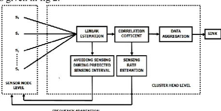
Hence, proposed scheme focuses on exploiting data correlation and predicting values at some future intervals so as to reduce energy consumption by eliminating redundant readings and tuning sensing frequency of SNs according to the nature of the event. The local estimation builds estimation model using linear regression analysis for each CH to estimate its readings. The CH gathers data from nodes under its control and finds correlation. Accordingly, it sets the sensing rate of SNs under its cluster. Thus, overall goal is to prolong the network life time by reducing inter-node transmissions and by tuning sensor frequencies. Overall abstract model of the scheme is given in fig 2.

Fig. 2. Abstract view of Proposed Adaptive Sensing Strategy

Next a complete strategy for linear estimation and sensing frequency adaptation is elaborated. First, local estimation at CH level is explained and subsequently a scheme to adaptively set sensing frequencies of SNs is given which exploits data correlation at CH level.

IV. L

E

In the local estimation model, past values can be used to predict current and future values. The sample to be predicted can be closely approximated as a linear combination of past samples. Linear regression analysis is used for predicting the future values from the past values buffered at CH. This model is capable of predicting data that evolves slowly over time and does not require a large amount of training data or a priori knowledge of the distribution of sensor values. Hence, it is suitable for CHs with limited computation capability.

Coefficient of regression of y on x =byx = 𝜇_𝜎11

𝑥2 =

𝑟 𝜎_𝑥 𝜎_𝑦 𝜎_𝑥2 =

𝑟 𝜎_𝑦

𝜎_𝑥 σx ≠ 0

By using the local estimation, a CH estimates newly generated readings through a data model learned from its historic data.

4.1 Sensing Frequency Adaptation

As per the dissemination model, every SN in a cluster sends the data to its CH. SN senses phenomenon after every small sensing interval (i.e. SNSI) determined by application requirements. If an event is detected, sensed data reading is pushed into SNbuffer. Once in each SNSI such sensed readings are periodically pushed into SNbuffer. When SNDI expires, SNbuffer disseminates buffered values to its CH. Thus, CH receives data values from all SNs in the cluster and pushes it to CHBUFFER. Based on these values, CH predicts data values for next SNDI interval and pushes it also into its CHBUFFER. At the beginning of the prediction interval, CH sends signal to SNs not to perform sensing and hence can go into sleep mode if SNDI is large enough, otherwise remain active without sensing. CH now has data in its buffer comprising readings sampled by SNs during a SNDI as well as predicted readings for next SNDI. Next, CH finds the correlation among the data values in its CHBUFFER. Let the variables (xi,yi ) occur with frequency fi ,(i=1,2,3,….n)

∑𝑛𝑖=1𝑓𝑖 =N

Therefore, the correlation coefficient is as follows rx,y =

1

𝑁 ∑ 𝑓𝑖(𝑥𝑖−𝑥̄)(𝑦𝑖−𝑦̄)

√_𝑁1∑ 𝑓_𝑖(𝑥_𝑖−𝑥̄)2 _√1

𝑁∑ 𝑓𝑖(𝑦𝑖−𝑦̄)2

r x,y = ∑ 𝑓𝑖 𝑥𝑖 𝑦𝑖− (1/𝑁) ∑(𝑓𝑖𝑥𝑖) ∑(𝑓𝑖𝑦𝑖) √∑ 𝑓_𝑖𝑥_𝑖2− (_𝑁1) (∑ 𝑓_𝑖𝑥_𝑖)2 _{√∑ 𝑓𝑖𝑦}

𝑖2− (𝑁1) (∑ 𝑓𝑖𝑦𝑖)2

The value of r is between -1 < r < +1. The + and – signs are used for positive linear correlations and negative linear correlations, respectively.

rate and transmitting it to CH, then a lot of redundant data is generated which is not useful. Thus, it wastes a lot of energy in unfruitful sensing and transmissions. To avoid this wastage of energy, sensing rate of SNs must be reduced (i.e. SNSI is increased) by some factor. When sensing frequency is reduced in steps, a situation arises when sufficient uncorrelated data readings arrive at CHbuffer. This indicates that sensing frequency has been reduced enough for relatively static event.

On the other extreme, if r is 0 then most of data readings are uncorrelated. This infers that event is highly dynamic and thus every reading sensed by sensors is different. This situation further suggests that we might be missing some important readings with existing sensing rate and thus sensing rate must be increased (i.e. SNSI to be reduced) to capture it. When sensing frequency is increased in steps, a situation arises when similar readings start buffering at CH implying thereby that sensing rate is sufficient enough not to miss important facts about the event.

But, there must be some limit for reducing and increasing the sensing frequency otherwise SNs will keep on altering sensing frequency between low and high. If we fix a single mid value (0.5) of r as limit, still to maintain r at this single value is impossible i.e. on slight change in the value on either side will necessitate the change in sensing frequency. Thus, to avoid this instability and conserve energy, we divide the overall state of the system into stable and unstable zones as per the table 1 below.

Table 1: Correlation coefficient and sensing rate CORELATION

COFFICENT (r)

SENSING RATE (SNSI)

UNSTABLE STATE

(NON CORRELATED

ZONE)

0 TO 0.3 SNSI=SNSI*(1+3

r)/2

STABLE STATE >0.3 TO <0.7 SNSI=SNSI

UNSTABLE STATE (CORRELATED

ZONE)

0.7 TO 1.0 SNSI=SNSI*(1+3

r)/2

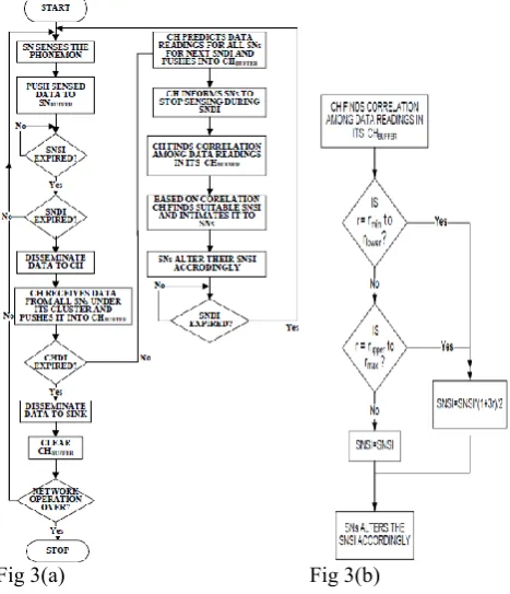
Sensing frequency is altered only when r is in unstable zone. It is clear that there exist two unstable zones: correlated zone and non-correlated zone. In both zones, SNSI is altered as follows:

SNSI=SNSI*(1+3r)/2

This is devised to ensure the fact that if r = 1, sensing frequency must be halved i.e. SNSI be doubled. For other values up to the limit 0.7 (rupper), the SNSI is altered

accordingly and at 0.7 it comes out to be 1.5 times SNSI. Similarly, if r = 0, sensing frequency must be doubled i.e. SNSI be halved. For other values up to the limit 0.3 (rlower), the SNSI is altered accordingly and at 0.3 it comes

out to be 0.9 times SNSI. For the values of r greater than 0.3 and less than 0.7, the correlation is neither weak nor strong. This state is stable state and SNs senses the event at normal sensing rate i.e SNSI. However, above function as well as values of rupper and rlower can be modified

according to the application requirement and can be made

scenario specific. When CHDI is over, CH sends the data to sink node and clears the CHBUFFER. Also, CH broadcasts this new SNSI value in its cluster for all SNs in the cluster to modify the value of SNSI accordingly. Thus, in order to reduce the overall energy consumption, the scheme adaptively controls the sensing rate of the SN by decreasing it when the data is correlated and increasing it otherwise. Flowchart in fig 3 gives detailed strategy

Fig 3(a) Fig 3(b)

V. P

E

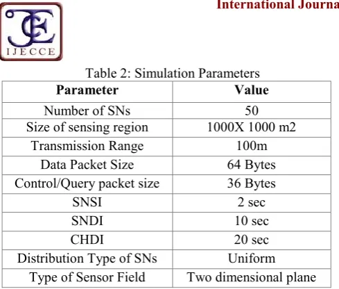
Table 2: Simulation Parameters

5.1. Number of Data Packets Transmitted

In this section, we evaluate the performance in terms of number of packets transmitted with varying node density. Fig 4 shows the number of packets transmitted with varying node density. The number of packets transmitted in ASDP is 16% less as compared to EEAST, Hybrid and ASAP respectively. This is because ASDP causes SNs to stop sensing for certain intervals of time as ASDP predicts the future values of SNs based on past values. Also, ASDP increases or decreases sensing rate of SNs depending upon the kind of events. Therefore, as the node density increases, more is the correlation among sensed values and thus sensing rate of SNs is accordingly decreased and thereby reducing the number of packets transmitted to CH and to sink node. Figure 4 shows comparison of number of data packets transmitted by different sensing strategies.

Fig. 4. Comparison of number of data packets transmitted

5.2. Number of Control Packets Transmitted

Fig 5 shows the number of control messages transmitted with time. The number of packets transmitted in ASDP is 12% more as compared to EEAST, Hybrid and ASAP respectively. This is because, ASDP increases or decreases sensing rate of SNs depending upon the kind of events. Therefore, as the node density increases, correlation among sensed values increases and hence sensing rate of SNs decreases and thereby reducing the number of packets transmitted. As number of data packets decreases, more numbers of control messages are transmitted. Fig 5 shows comparison of number of control packets transmitted by different sensing strategies.

Fig. 5. Comparison of number of control packets transmitted

5.3. Overall Network Energy Consumption

In this section, we evaluate the performance in terms of energy consumption with time. Fig 6 shows the overall energy consumption with time. The overall energy consumption of ASDP is 10% less as compared to EEAST, Hybrid and ASAP respectively. This is because ASDP causes SNs to stop sensing for certain intervals of time as ASDP predicts the future values of SNs based on past values. Also, ASDP increases or decreases sensing rate of SNs depending upon the kind of events. Therefore, as the node density increases, the more and more correlation between the sensed values and less will be the sensing rate of SNs and thereby reducing the number of packets transmitted to SN and thereby to sink node and thereby reducing the energy consumption of SNs. Fig 6 shows the total energy consumption comparison of different adaptive sensing strategies.

Fig. 6. Overall Energy consumption of different sampling algorithms

VI . C

F

W

The proposed Adaptive Sensing for Energy Efficient Data Dissemination (ASDP) finds adaptive sensing rate for SNs. To do this, the scheme utilizes the local estimation at every CH and finds correlation among these sensed values at CH level. The local estimation builds estimation model using linear regression analysis for each

Parameter Value

Number of SNs 50

Size of sensing region 1000X 1000 m2

Transmission Range 100m

Data Packet Size 64 Bytes

Control/Query packet size 36 Bytes

SNSI 2 sec

SNDI 10 sec

CHDI 20 sec

Distribution Type of SNs Uniform

CH to estimate its readings and reduces the communication cost between each SN and its CH. The

nodes after sensing the data send it to CH. The CH gathers data from SNs under its control and estimates new value using local estimation model and then finds correlation among sensed values. Accordingly, it adaptively sets the sensing rate of SNs under its cluster. Analytical and simulation study reveals significant improvement in term of transmission cost and total energy consumption. The performance of proposed ASDP scheme is better than existing similar schemes.

There are few directions for future research. First, our scheme controls the sensing rate of SNs. More sophisticated cost model that takes other factors, such as queuing effect and link quality, into consideration shall be further studied. Also, it is a long-term goal to design an efficient protocol that acts dynamically to any topology change in a wireless network for an optimal sensing rate of SNs.

R

[1] I.F. Akyildiz, M.C. Vuran, O. Akan, W. Su: “Wireless Sensor Networks: A Survey Revisited” In: Computer Networks Journal (Elsevier Science), Vol. 45, no. 3, 2004

[2] K. Akkaya, M. Younis: “A Survey on Routing Protocols for Wireless Sensor Networks” In: Elsevier Ad Hoc Network Journal, Vol. 3, pp. 325- 349, 2005.

[3] S. Olariu, Q. Xu, A. Zomaya, “An energy-efficient self-organization protocol for wireless sensor networks”, in: Intelligent Sensors, Sensor Networks and Information Processing Conference (ISSNIP), IEEE, Melbourne, Australia, 2004, pp. 55–60.

[4] H.S. Abdel Salam, S. Olariu, “A lightweight skeleton construction algorithm for self-organizing sensor networks”, in: ICC, IEEE, 2009, pp. 1–5.

[5] C. Guestrin, P. Bodi, R. Thibau, M. Paski, and S. Madde, “Distributed Regression: An Efficient Frame Work for Modeling Sensor Network Data”, Proc. Third Int’l Symp. Information Processing in Sensor Network (IPSN), 2004.

[6] Ge-Ming Chiu, Li-Hsing Yen and Tai-Lin Chin“Optimal Storage Placement for Tree-Structured Networks with Heterogeneous Channel Costs ”,IEEE Transactions on computers, Vol. 60, NO. 10, October 2011.

[7] I. Chatzigiannakis, T. Dimitriou, S.E. Nikoletseas, P.G. Spirakis, “A probabilistic algorithm for efficient and robust data propagation in wireless sensor networks”, Ad Hoc Networks 4 (5) (2006) 621–635.

[8] C. Intanagonwiwat, R. Govindan, and D. Estrin. “Directed Diffusion: A Scalable and Robust Communication Paradigm for Sensor Networks”, in Proc. of ACM MobiCom, 2000.

[9] S. Madden, W. Hong, J. M. Hellerstein, and M. Franklin. TinyDB web page: http://telegraph.cs.berkeley.edu/tinydb. [10] Y. Yao and J. Gehrke. “Query Processing in Sensor Networks”,

in Proc. CIDR, 2003.

[11] E. Shih, S.-H. Cho, N. Ickes, R. Min, A. Sinha, A. Wang, A. Chandrakasan, “Physical layer driven protocol and algorithm design for energy-efficient wireless sensor networks”, in: Proceedings of the 7th Annual International Conference on Mobile Computing and Networking, MobiCom ’01, ACM, New York, NY, USA, 2001, pp. 272–287.

doi:http://doi.acm.org/10.1145/381677.381703. <http:// doi.acm.org/10.1145/381677.381703>.

[12] I. Chatzigiannakis, T. Dimitriou, S.E. Nikoletseas, P.G. Spirakis, A probabilistic algorithm for efficient and robust data propagation in wireless sensor networks, Ad Hoc Networks 4 (5) (2006) 621–635.

[13] I. Chatzigiannakis, S. Nikoletseas, P.G. Spirakis, Efficient and robust protocols for local detection and propagation in smart dust

networks, Mobile Networks & Applications 10 (1–2) (2005) 133–149.

doi:http://doi.acm.org/10.1145/1046430.1046441.

[14] C. Efthymiou, S. Nikoletseas, J. Rolim, Energy balanced data propagation in wireless sensor networks, Wireless Networks 12 (6) (2006) 691–707. doi:http://dx.doi.org/10.1007/s11276-006-6529-y.

[15] Leandro A. Villas , Azzedine Boukerche, Horacio A.B.F. de Oliveira “A spatial correlation aware algorithm to perform efficient data collection in wireless sensor networks”ELSEVIER Journel Ad Hoc Networks 12 (2011) 69–85

[16] A. Jain and E. Y. Chang, “Adaptive sampling for sensor networks,” in Proc. Workshop DMSN, Toronto, ON, Canada, 2004, pp. 10–16.

[17] Cesare Alippi, iuseppe Anastasi, Mario Di Francesco, and Manuel Roveri “An Adaptive Sampling Algorithm for Effective Energy Management in Wireless Sensor Networks With

Energy-Hungry Sensors ”IEEE TRANSACTIONS ON

INSTRUMENTATION AND MEASUREMENT, VOL. 59, NO. 2, FEBRUARY 2010.

[18] P. Padhy, R. K. Dash, K. Martinez, N. R. Jennings, “A utility-based adaptive sensing and multihop communication protocol for wireless sensor networks”, ACM Transactions on Sensor Networks (TOSN), Volume 6 Issue 3, June 2010 No. 27 ACM New York, NY, USA

[19] S. Chatterjea, and P.J.M Havinga, "An Adaptive and Autonomous Sensor Sampling Frequency Control Scheme for Energy-Efficient Data Acquisition in Wireless Sensor Networks. In: 4th IEEE International Conference on Distributed Computing in Sensor Systems (DCOSS), 11-14 Jun 2008, Santorini, Greece. pp. 60-78.

[20] A.L. Wood, G. V. Merrett, S. R. Gunn, B.M. Al-Hashimi, N.R. Shadbolt, and W. Hall, “Adaptive sampling in context-aware systems: a machine learning approach.” IET Wireless Sensor Systems 2012,London, Jun 2012.

[21] D.N. Nkwogu and A.R. Allen “Adaptive Sampling for WSAN Control Applications Using Artificial Neural Networks” Journal of Senor and Actuator Networks 2012, 1(3), 299-320

[22] Alireza Masoum, Nirvana Meratnia, Paul J.M. Havinga “ An Energy-Efficient Adaptive Sampling Scheme for Wireless Sensor Networks” IEEE ISSNIP 2013.

[23] T.P. Sharma, R.C. Joshi, Manoj Misra, “Data Filtering and Dynamic Sensing for Continuous Monitoring in Wireless Sensor Networks,” in the special issues of International Journal of Autonomous and Adaptive Communications (IJAACS), vol. 3, no. 3, pp. 239-263, 2010.

A

'

P

Vipan Arora have done B. Tech from NIT Hamipur (H.P), India and M.Tech from DAVIET, Jalandhar. Presently he is pursuing PH.D. from NIT Hamirpur (H.P.). He is presently working as Head Computer Engineering department at Government Polytechnic College for girls, Jalandhar, Punjab, India. He has authored more than 25 books. His areas of interest includes adhoc and sensor networks

Dr. T. P. Sharma have done doctorate from IIT, Roorkee. He is presently working as Associate professor, NIT Hamirpur (H.P.). He has authored more than 70 papers in renowned International Journals. He has guided 5 PHDs and number of M Tech students. His areas of interest includes clustering, adhoc and sensor networks.