journal homepage: http://jac.ut.ac.ir
Changes in Artificial Neural Network Learning
Parameters and Their Impact on Modeling Error
Reduction
Somayeh Mehrabadi
∗ABSTRACT ARTICLE INFO
The main objective of this research is to investigate the effect of neural network architecture parameters on model behavior. Neural network architectural factors such as training algorithm, number of hidden layer neu-rons, data set design in training stage and the changes made to them, and finally its effect on the output of the model were investigated. It developed a database for modeling using by multi-layer perceptron. In particular, the modeling process enjoyed three training algorithms: Bayesian Regularization (BR), Scaled Conjugate Gradi-ent (SCG) and Levenberg Marquardt (LM). Model se-lection criteria based on the lowest error rate and data regression, using a trial and error approach. The results showed that models that greatly reduce the error have less generalizability. In the meantime, the BR algorithm with the data set design of 15-15-70 (for test, validation and training sections, respectively), has been used to reduce the error better than other algorithms,
Article history:
Received 30, April 2018
Received in revised form 10, October 2018
Accepted 18 November 2018 Available online 30, December 2018
Keyword: Artificial Neural Network, Learning Parameter,
Modeling
AMS subject Classification: 05C80.
∗Corresponding author: S. Mehrabadi. Email: [email protected]
1
Abstract continued
but improper generalizability. In contrast, the LM algorithm has better generalizability than the other two algorithms. Data analysis shows that, in most cases, when the amounts of data dedicated to test and validation change (increase or decrease), the model requires more neurons in order to reduce errors.
2
Introduction
People‘s ability to learn is different, so it‘s important to use time, tools and methods to teach a subject for some people. It depends on the ability of each person‘s brain to learn. The neuron is an irradiated cell that processes and transmits information by sending an electrical and chemical signal. Like the nervous system of the brain, an artificial neural network consists of a connected network of neurons with simple processing units.[8] These changes are influenced by training parameters in the artificial neural network and occur in a defined mathematical function. Among the parameters of these functions are data and its combinations, training algorithm, number of neurons, transfer function. In other words, the created weights are similar to chemical and electrical signals in the neural network of the brain.
effective parameters of the neural network training, especially training algorithms. Here, this study reports briefly the literature that it found. Neural networks are able to analyze multi-source datasets and they are considered as general approximations. [12]
3
Theory / calculation
3.1
Modeling
An artificial neural network uses computer technology to model a biologic neural system both structurally and functionally. [15] For modeling, has been used multi-layer perceptron neural model. The perceptron network uses the transfusion capabilities of the brain cells, it takes the input signal and makes it to the output, this is the mathematical explanation of a neuron. [21] Furthermore, the degradation parameters were introduced as the input and the numerical values referring to the degraded and non-degraded areas were introduced as the output. The modeling was performed using different training data set design and the three algorithms of Levenberg Marquardt (LM), Bayesian Regularization (BR) and Scaled Conjugate Gradient (SCG), and also different number of neurons, and finally the results were obtained.
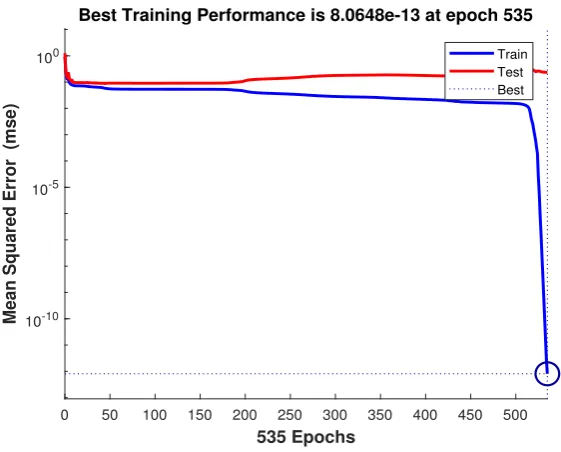
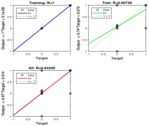
In the perceptron network the inputs are multiplied by the connection weights are first summed and then, are transmitted to a transfer function to give output for that neu-ron. The transfer function included (purelin, hardlim, sigmoid, logistic) executes on the weighted sum of the neurons inputs. [20] Each input is a multiplicative of the weight coefficients that are summed up eventually. Activation function determines the proper-ties of the artificial neuron.[18] Neural Networks consist of coefficients or weights in a neural network structure. [11] This paper is used sigmoid hidden neurons and linear out-put neurons. The figures 1,2,3 & 4 represent the final model outout-put, contains: training performance, error histogram, regression and training state.
0 50 100 150 200 250 300 350 400 450 500
535 Epochs
10-10 10-5 100
Mean Squared Error (mse)
Best Training Performance is 8.0648e-13 at epoch 535
Train
Test
Best
0 20 40 60 80 100 120 140 160 180 Instances
Error Histogram with 20 Bins
-0.95 -0.85 -0.75 -0.65 -0.55 -0.45 -0.35 -0.25 -0.15 -0.05 0.05 0.15 0.25 0.35 0.45 0.55 0.65 0.75 0.85 0.95
Errors = Targets - Outputs
Training Test Zero Error
Figure 2: In figure 2 , the error histogram shows the error in the test and training datasets, and they differ only in the last stages.
-1 -0.5 0 0.5 1
Target -1 -0.5 0 0.5 1
Output ~= 1*Target + 3.1e-08
Training: R=1
Data Fit Y = T
-1 -0.5 0 0.5 1
Target -1 -0.5 0 0.5 1
Output ~= 0.74*Target + 0.075
Test: R=0.60736
Data Fit Y = T
-1 -0.5 0 0.5 1
Target -1 -0.5 0 0.5 1
Output ~= 0.97*Target + 0.014
All: R=0.93258
Data Fit Y = T
10-10 100 1010
gradient
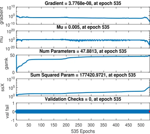
Gradient = 3.7768e-08, at epoch 535
10-20 100 1020
mu
Mu = 0.005, at epoch 535
0 50
gamk
Num Parameters = 47.8813, at epoch 535
100 105 1010
ssX
Sum Squared Param = 177420.9721, at epoch 535
0 50 100 150 200 250 300 350 400 450 500 535 Epochs
-1 0 1
val fail
Validation Checks = 0, at epoch 535
Figure 4: In this figure, Neural network configuration parameters are specified.
3.2
Data
In this study, has been used remotely sensed data to detect changes in Mazandaran forest, particularly the forest cover around Sari, located in north of Iran, over fifteen years (1999 2014). Our tools for capturing the forest state include Landsat-5 TM sensor for 1999 and Landsat 8 OLI sensor for 2014. Further, for extracting geographical information of the degradation parameters, it used Irans National Cartographic Center maps.
3.3
Database Creation
4
Results
4.1
Conducting comparisons
(Before explaining comparisons, it is worthwhile to mention that the results and tables, here, represent the analysis of the best outcomes in terms of the type of training algorithm, the number of hidden layer neurons and the training data set design. So, it conducts comparisons among the best outcomes and discussing others is to be avoided.)
In this paper the researche used three training algorithms (LM, BR and SCG) with different number of neurons and 5 different data set designs, including (65-15-20/65-20-15/75-10-15/75-15-10/70-15-15).
After analyzing and selecting the best models in terms of reducing the error rate and also overall regression, such models were further analyzed and compared based on the type of training algorithm, data set design and number of hidden layer neurons.
The results are as follows:
The first comparison aimed at selecting an appropriate model based on the type of training algorithm;
In the process of leering a training algorithm is used to update network weights by com-paring Comparison between the obtained output and the target output then it modifies systemically the weight throughout the network till it finds the optimum weights ma-trix. [16] The performances of the learning algorithms are evaluated by comparing the convergence speed and the prediction error. [17]
Algorithm locates the minimum of a multivariate function that can be expressed as the sum of squares of non-linear real-valued functions. It is an iterative technique that works in such a way that performance function will always be reduced in each iteration of the algorithm. This feature makes trainlm the fastest training algorithm for networks of moderate size. [20]
Using error reduction and overall regression as the criteria for selecting the appropriate model, it found that the Bayesian Regularization algorithm put forward the best perfor-mance in reducing error rate and enhancing regression rate, which shows the harmony of training data set design.
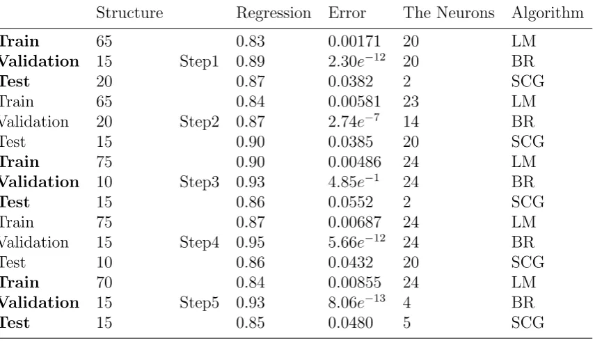
The Table 1 represents the results.
As table 1 demonstrates, the number of hidden layer neurons, as a non-critical factor here, varies between 2 to 24 and, nevertheless, the model has achieved the appropriate results. Considering the performance for the 5 different data set designs, regardless of the number of neurons, the LM training algorithm was the second best and the SCG was the third. Moreover, the second comparison aimed at selectinga model based on the best train-ing data set design (traintrain-ing, validation and test);
Table 1: Comparison Results of the 5 Different Data set Designs for the Three Algorithms of LM, BR and SCG with Different Amount of Hidden Layer Neurons
Structure Regression Error The Neurons Algorithm
Train 65 0.83 0.00171 20 LM
Validation 15 Step1 0.89 2.30e−12 20 BR
Test 20 0.87 0.0382 2 SCG
Train 65 0.84 0.00581 23 LM
Validation 20 Step2 0.87 2.74e−7 14 BR
Test 15 0.90 0.0385 20 SCG
Train 75 0.90 0.00486 24 LM
Validation 10 Step3 0.93 4.85e−1 24 BR
Test 15 0.86 0.0552 2 SCG
Train 75 0.87 0.00687 24 LM
Validation 15 Step4 0.95 5.66e−12 24 BR
Test 10 0.86 0.0432 20 SCG
Train 70 0.84 0.00855 24 LM
Validation 15 Step5 0.93 8.06e−13 4 BR
Test 15 0.85 0.0480 5 SCG
a) 20-15-65 (for test, validation and training sections, respectively) training data structure with 20 number of neurons for LM algorithm.
b) 15-15-70 (for test, validation and training sections, respectively) training data structure with 4 number of neurons for BR algorithm.
c) 15-20-65 (for test, validation and training sections, respectively) training data set design with 20 number of neurons for SCG algorithm. Tables 2, 3 and 4 also show the results.
Table 2: Different data set designs with different amount of hidden layer neurons for the LM algorithm.
Total Regression Error The Neurons of Hiden Structure
Test Validation Train
0.83 0.00171 20 20 15 65
0.84 0.00581 23 15 20 65
0.90 0.00486 24 15 10 75
0.87 0.00687 24 10 15 75
0.86 0.00406 25 15 15 70
According to Table 2, with 20 hidden layer neuron, the LM algorithm had the best performance when the amount of training data was reduced and the amount of test data was increased (comparing to the final model with the design of 70-15-15).
regres-Table 3: Different data set designs with different amount of hidden layer neurons for the BR algorithm.
Total Regression Error The Neurons of Hiden Structure
Test Validation Train
0.89 2.3e−12 20 20 15 65
0.87 2.76e−7 14 15 20 65
0.93 4.85e−12 24 15 10 75
0.95 5.66e−12 24 10 15 75
0.93 8.06e−13 4 15 15 70
sion increase, the BR algorithm outperform the SCG and LM. However, in most cases, this yielded as the result of an increase in the number of neurons, except when the amount of test and validation data were equal. In addition, according to table 3, the BR algorithm had the best performance when the test and validation data were equal (15 for both).
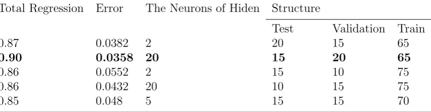
Table 4: Different data set designs with different amount of hidden layer neurons for the SCG algorithm
Total Regression Error The Neurons of Hiden Structure
Test Validation Train
0.87 0.0382 2 20 15 65
0.90 0.0358 20 15 20 65
0.86 0.0552 2 15 10 75
0.86 0.0432 20 10 15 75
0.85 0.048 5 15 15 70
Table 4 further shows that when the amount of validation and training data increased and also when the amount of test and validation data were equal, SCG algorithm put forward a satisfactory result with decreasing the number of neurons. On the other hand, when the amount of test data were equal or more than the validation data, SCG were able to run the model properly with decreasing the number of neurons. The conjugate gradient algorithm is faster than other algorithms but the results are not without problems. [6] As can be seen in Table 4, with 20 hidden layer neuron, the best training data set design for the SCG algorithm has achieved when the amount of validation data was increased and the amount of training data was decreased (comparing to the final model 70-15-15). And finally the third comparison aimed at selecting an appropriate model based on the least number of neurons;
set tends to be a small number. [23] For this purpose, the same number of neurons was used for the algorithms. Then, the best model was selected based on the lowest error rate, the highest overall regression and the least number of hidden layer neurons. The results showed that the SCG put forward the best performance in reducing the number of neurons, comparing to the other two algorithms. Accordingly, the best model for the SCG algorithm was obtained with 2 neurons, for the BR algorithm with 4 neurons and for the LM algorithm with 20 neurons. Tables 5, 6, 7, 8 and 9 show the results.
Table 5: The comparing the results of the three algorithms for 65-20-15 Error Regression Neurons Algorithm Structure
0.00581 0.84 23 LM Test Validation Train
2.74e−7 0.87 14 BR 15 20 65
0.0358 0.90 20 SCG
According to Table 5, the three algorithms produced appropriate results with an increase in the number of neurons. Nevertheless, BR algorithm provided appropriate results with the least number of neurons, comparing to others.
Table 6: The comparing the results of the three algorithms for 65-15-20. Error Regression Neurons Algorithm Structure
0/00171 0.83 20 LM Test Validation Train
2.30e−12 0.89 20 BR 20 15 65
0.0382 0.87 2 SCG
Considering the dataset design represented in Table 6, among BR, SCG and LM algo-rithms, SCG had an appropriate performance in running the model with the least number of neurons, but, on the other hand, LM and BR did the same with significantly higher number of neurons.
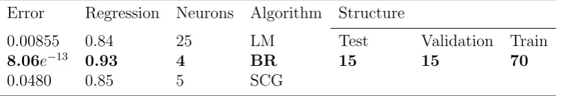
Table 7: The comparing the results of the three algorithms for 70-15-15. Error Regression Neurons Algorithm Structure
0.00855 0.84 25 LM Test Validation Train
8.06e−13 0.93 4 BR 15 15 70
0.0480 0.85 5 SCG
Table 8: The comparing the results of the three algorithms for 75-10-15. Error Regression Neurons Algorithm Structure
0/00687 0.87 24 LM Test Validation Train
5.66e−12 0.95 24 BR 15 10 75
0.0432 0.86 2 SCG
In the dataset design represented in Table 8, SCG had the best performance with the least number of neurons. According to this table, the number of neurons in BR and LM were equal, however, it shows a great difference from SCG (2 neurons comparing to 24).
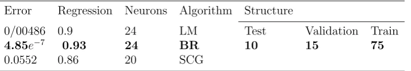
Table 9: The comparing the results of the three algorithms for 75-15-10. Error Regression Neurons Algorithm Structure
0/00486 0.9 24 LM Test Validation Train
4.85e−7 0.93 24 BR 10 15 75
0.0552 0.86 20 SCG
In Table 9, in which it utilized a different dataset design, again, SCG algorithm had the best performance in modeling using the lowest number of neurons. The other two algorithms provided appropriate results with 24 number of neurons. Despite the pervious run represented in Table 8, the difference in the number of neurons between the three algorithms was not significant.
4.2
Changing the data set designs and observing the effects on
algorithm outputs
the amount of training, and also reducing the amount of validation and again increasing the amount of training data in this form: 75-10-15 and 75-15-10 for training, validation and test data respectively. After analyzing the results, it was found that when the amount of validation data is reduced and training data amount increased, the number of hidden layer neurons increased in case of using LM and BR algorithms (24 neurons for both) and decreased in case of using SCG algorithm (2 neurons). On the other hand, utilizing the data set design of 75-15-10, when it reduced the amount of test data and increased the amount of training data, it rose the number of neurons in all three algorithms. Taking into consideration all the effective factors (error reduction, overall regression, number of neurons and data set design), this paper found that the BR algorithm is the best choice than the LM or SCG. However, it should be noted that the SCG algorithm has also a successful performance in reducing the number of neurons and, as a result, reducing errors.
5
Conclusion
Generally, the comparisons show that, in most cases, when the amounts of data dedi-cated to test and validation change (increase or decrease) comparing to the best data set design (70-15-15 for training, validation and test, respectively), the model requires more neurons in order to reduce errors. Actually, it obtained the best result for the algorithms by increasing the number of hidden layer neurons. Basically, regarding neural network architectures, optimal results are not usually obtained by increasing the number of hidden layer neurons. In fact, increasing the hidden layer neurons would make the processes more complex which may, as a result, increase the risk of achieving unrealistic and unreliable findings.
algorithms, analyzing the absolute values of error for all the models in this study show that differences between these error rates are very small and can be ignored.
Consequently, it cannot question the suitability of the Levenberg Marquardt and Scaled Conjugate Gradient algorithms for modeling. This article explained that, taking into consideration the accuracy of the input data and the researchers expectation of output accuracy of the model, artificial neural network is one of the best approaches for modeling forest degradation and investigating degradation effective parameters. In conclusion, it can be said that the Bayesian Regularization algorithm is more suitable and put forward a better performance than the LM & SCG algorithms in modeling nonlinear natural phe-nomena and modeling using multi-layer Perceptron (MLP) neural network. The results showed that models that greatly reduce the error have less generalizability. In the mean-time, the BR algorithm has been used to reduce the error better than other algorithms, but improper generalizability. In contrast, the LM algorithm has better generalizability than the other two algorithms.
References
[1] Akbarzadeh, A., Taghizadeh Mehrjardi, R., Rouhipour, H., Gorji, M., Refahi, H. Estimating of Soil Erosion Covered with Rolled Erosion Control Systems Us-ing Rainfall Simulator (Neuro-fuzzy and Artificial Neural Network Approaches).
J ournalof AppliedScienesResearch. (2009).5, 505-514.
[2] Akkar, D. A., Firas, M. R. Evolutionary Algorithms For Neural Networks Binary And Real Data Classification. InternationalJ ournalOf Scientif ic&T echnologyReserch. 5(7) (2016) 55-60.
[3] Al-Hmouz, A., Shen, J., Senior Member IEEE, Al-Hmouz, R., Yan, J. Modeling and Simulation of an Adaptive Neuro-Fuzzy Inference System (ANFIS) for Mobile Learning.
IEEET ransactionsonLearningT echnologies . 5(3) (2012) 226-237.
[4] Ayat, S., Farahani, H. A., Aghamohamadi, M., Alian, M., Aghamohamadi, S., Kazemi, Z. A comparison of artificial neural networks learning algorithms in pre-dicting tendency for suicide. N euralComputing&Application . 23, (2013) 1381-1386. doi:10.1007/s00521-012-1086-z
[5] Bashiri, M., FarshbafGeranmayeh, A. Tuning the parameters of an artificial neural network using central composite design and genetic algorithm. ScientiaIranica .18 (2011) 1600-1608.
[6] Fletcher, R., Reeves, C. M. Function minimization by conjugate gradients.
T hecomputerjournal . 7(2) (1964).
[8] Guerriere, M. R., Detsky, A. S. Neural Networks: What Are They? Annals Of Internal Medicine. 11 (1991)
[9] Gunther, F., Fritsch, S. neuralnet: Training of Neural Networks. T heRJ ournal . 2 (2010)
[10] Gupta, J. N., Sexton, R. S. Comparing backpropagation with a genetic algorithm for neural network training. OMEGA, T heInternationalJ ournalof M anagementScience
. (1999) 679-684.
[11] Haykin, S. NEURAL NETRORKS : A Comprehensive Foundation (2 ed.). (p. hall, Ed.) pearson. (1999)
[12] Horinik, K. Approximation Capabilities Of Multilayer Feedforward Networks.
N euralN etwork . 4 (1991)
[13] Hyvarinen, A., Oja, E. Independent component analysis: algorithms and applica-tions.N euralN etworks . 13 (2000) 411430.
[14] Ilonen, J., Kamarainen, J.-K., Lampinen, J. Differential Evolution Training Algo-rithm for Feed-Forward Neural Networks. N euralP rocessingLetters . 17 (2003) 93-105.
[15] Itchhaporia , D., Snow , P. B., Almassy , R. J., Oetgen , W. J. Artificial Neural Networks: Current Status in Cardiovascular Medicine.J ACC . 28 (1996) 515-521. [16] Mahmoud, O., Anwar, F., Jimoh, M., Salami, E. Leraning Algorithm Effect On
Multilayer Feed Forward Artificial Neural Network Performance In Image Coding.
J ournalof EngineeringScienceandT echnology . (2007) 188-199.
[17] Nouir, Z., Sayrac, B., Fouresti, B., Telecom, F., Division, R. Comparison of Neural Network Learning Algorithms for Prediction Enhancement of a Planning Tool,. 38 rue G eral Leclerc Issy-les-Moulineaux FRANCE.(2010)
[18] Rojas, R. Neural Networks A Systematic Introduction. Springer. (1996) 429-449. [19] Rumelhart, D. E., Hinton, G. E., Williams, R. J. Learning Internal Representations
By Error Propagation. 1 (1986)MIT Press Cambridge.
[20] Sharma, B., Venugopalan, P. Comparison of Neural Network Training Functions for Hematoma Classification in Brain CT Images.J ournalof ComputerEngineering . 16(1) (2014) 31-35.