On the distribution of the error of an interpolated value, and on the construction of tables

(1)

On the Distribution of the Error of an Interpolated Value, and on the Construction of Tables. By R. A. FISHER, SC.D., Gonville and Caius College, and Mr J. WISHART.

[Received 8 August, read 24 October 1927.] 1. Introduction.

Before the introduction of interpolation formulae, beyond linear interpolation by proportional parts, the presentation of the numerical values of mathematical functions was much restricted, for the labour of computation and the cost of printing, to say nothing of the inconvenience of handling a bulky volume, had to be increased quite disproportionately with every increase in accu-racy. A four-figure logarithm table occupies two small pages, Chambers's seven-figure table takes 150 pages, while Vega's ten-figure table requires 300 pages twelve inches long.

The modern tendency towards compact tables used with more or less high order interpolation formulae arises from two advances: (i) the introduction of simple and adequate interpolation formulae, and (ii) the development of the theory of the remainder term. The central difference formulae of Everett not only reduce the calculation of the interpolate to a few very simple operations, of a kind suitable for machine calculations, but since they require only even differences they enable adequate differences to be presented compactly with the table. Tables of the coefficients of the second, fourth and sixth differences have been prepared by A. J. Thompson (1,1921). Even a moderate use of differences results in a very great saving. For example in A. J. Thompson's recent twenty-figure logarithm tables (2) the values from *9 to TO occupy only 100 pages, although differences beyond the second are not required, the fourth differences being negligible. The table could in fact have been made much more compact, by the use of higher differences, although in view of the special properties of the logarithm, it is doubtful if this would be desirable. Pearson has exhibited seven-figure logarithm and anti-logarithm tables which, using second differences, together occupy only a single page (3,1920, p. 60).

(2)

tabulated, and if so an interpolation formula will give the inter-polate to the full accuracy of the table. A table should in fact always be regarded as giving not an isolated series of values of a function, but, by means of the interpolate function implicit in these, the whole continuum of its values. The possibility of ade-quate interpolation thus depends on the tabular intervals being sufficiently small for the remainder term to be negligible. This condition allows of the use of immensely more compact tables than the requirement that linear interpolation shall be valid, and brings with it the possibility of accurate tables of double and triple entry, without prohibitive labour either in their preparation or their use.

When the remainder term is negligible the error of the inter-polate will depend only on the tabular errors, that is to say, on the differences between the exact value of the function and the corre-sponding value given in the table. When a table is "correct to the last figure " this error will be uniformly distributed between the limits — 0"5 and + 0"5 in the last place. Disproportionate efforts are often made to ensure this accuracy of the last place. Calculations are frequently carried to two or three figures more than are given in the final form, and the entries then cut down. Even so, it is by no means certain, owing to entries occurring that end in 50 or 500, that the final figure will in all cases be "correct"; and a lengthy series of calculations in such a doubtful case will seldom effect more improvement than to replace an error of say '503 by one of '497, a most trifling gain seeing that the standard error of a "correct" table is -288. It has not been hitherto sufficiently realised that a table to a larger number of places, the last one or two of which are not necessarily correct, is capable of giving a more accurate interpolate than the same table cut down, provided that the standard error of the tabular entry is known. The expense of printing one or more figures would be more than compensated for by the increased accuracy obtainable. It is usually possible to ensure that positive and negative errors should be, in the long run, equally frequent, and that the distribution of errors shall follow approximately the normal law.

(3)

i.e. no correlations exist between e, and e2, e, and e3, etc., where e

denotes the error of a single value. All the formulae of interpola-tion by differences are included in the following general reasoning, where Lagrange's formula has been used, and the intervals assumed, for simplicity, to be equal.

2. The Mean Variance of the Interpolate.

Let p be the fraction of the interval (taken as 0 to 1) for which it is desired to obtain an interpolated value. Let q = 1 — p. Then we shall examine the contribution of any one error to the variance of the interpolate for one-, two-, three-, four- point formulae and average this over the interval. The total contribu-tion will be expressed as a polynomial in pq and we shall use the result that

l-point Interpolation.

The interpolate is here equal to the tabular entry, and so the ratio of the variance of the interpolate to that of the entry is unity.

2-point Interpolation.

We have contributions qe at 0 and pe at 1. The variance of the interpolate is then the average value of

(p' + q*)a' = (l and our required ratio is | .

3-point Interpolation.

Contributions to the error are

a n d

We then have the total variance

= ^ [(1 - 4pg) (5 - 4pg) + 2 (3 + 4pqYl

and the average value of the variance of the interpolate is 429 „

480 *'

(4)

A similar procedure gives, for 4-point interpolation, '77566, 5-point -89574, 6-point -82244, 7-point -90291, and 8-point -84942.

3. The Limiting Condition for High Order Interpolation.

It is easy to show that the limit to the ratio of variances as the number of points is indefinitely increased must be unity. For the function

(x - a,) (x - a,) (x - Op-,) (x - ap+1) (x-an)

(ap-a1){ap-a2) (ap - a^) (ap - ap+1) {ap-an)

vanishes at all points a1( a?, an except ap, at which its value

is unity. When n is large, and the intervals equal to unity, the function tends to resemble

sin ir(x — ap)

7r(x- ap)

The average contribution of any one error to the variance of the interpolate is then

- dx, where x = — ,

—2j--av ™

-ae,

and the average value of the total variance, expressed as a ratio to that of the tabular entry, will be

sin20,- lrsin

_w

2^]0 0 , I f 2sin0cos0,,.

L J

+

— o —

d d

>

of which the first term vanishes, while the second is

I f sin ft

J±

— I —-r1- ad> = 1. ("I)

7TJ - o o <f>

We have, then, the result that the average standard error of the interpolate is always somewhat less than that of the tabular entry, being least for linear interpolation, and the advantage of a system of tabulation which is not concerned with the accuracy of the last figure recorded, but which states the standard error of entry, is apparent.

(5)

errors will be exactly the same as for 2-point interpolation. This condition is nearly realised when even differences are given correct to the last digit of the tabular values.

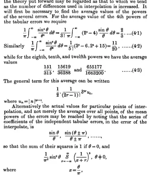
4. The Error Distribution for High Order Interpolation. When we turn to examine not merely the variance but the form of the distribution of the error in the interpolate, a normally distributed tabular error is seen to have an added advantage beyond that due to the increased accuracy attainable when the table is not cut down to be " correct to the last place." In what follows n, the number of points, will be assumed to be large, and the theory put forward may be regarded as that to which we tend as the number of differences used in interpolation is increased. I t will first be necessary to find the average values of the powers of the several errors. For the average value of the 4iih powers of the tabular errors we require

Similarly I J ^ ^<0== l(3°-6.2»+15)=|-J, (2)

while for the eighth, tenth, and twelfth powers we have the average values

151 15619 655177

315' 36288 1663200' K }

The general term for this average can be written 2-(2r-l)!

where un = | n I59""1.

Alternatively the actual values for particular points of inter-polation, and not merely the averages over all points, of the mean powers of the errors may be reached by noting that the series of coefficients of the independent tabular errors, in the error of the interpolate, is

sin 0 sin (0 ± ir)

so that the sum of their squares is 1 if 8 = 0, and

1 oo / 1 S3

-±-sin0 8 [ — ) , 00,

7T2 r=_oo \x+rj

(6)

and r is an integer. We have

Also

J

[(x — 1)! is written for T(x) even though x is not an integer.] Adding, we have

Thus the sum of squares is unity for all values of 0. The sum of the fourth powers is, similarly,

1 3s

o ls i n 4 0 ^ (cosec2 0) = 1 - 1 sin2 0 (4-4)

o! otf

For the sixth powers we have

l - s i n ^ + ^sin'fl, (4-5) and for the eighth powers

n80 (4'6)

These expressions are the coefficients of h2, h*, etc., in the ex-pansion of

hx cot (0 — hx), where x — sin 0.

The assumption is made that the error distribution of the interpolate will be symmetrical, so that only even moments need be considered. The two cases that arise are (a) normal distribution of tabular errors, which occur when the table is used as constructed, and not cut down, (b) rectangular distribution of errors, as in the case of all ordinary tables, which are correct to the last figure. So that in (6) if dp- represent the small element of frequency (=f(x) dx), we have dp = dx for all values of x between — £ and + £, say, and dp = 0 outside these limits.

The nature of the distributions is best exhibited by studying their characteristic functions. If, in the usual notation,

fir' = I xrdp J - 0 0

(7)

moment about the mean, then the Moment Generating Function is defined as

M=

4 _{+ /}

4 ₊

) (4-7)

The logarithm of M may be called the Kappa Generating Function, and we have

K = logif = Klt + * , | j + «, | j + .,...., (4-8) where the K'S are the semi-invariants of Thiele. Thus

*i = /V, «2 = M2, ic3 = f*3, * 4 = M 4 - 3 ^2, Kh = us - 10/i2/i3, etc.

An important property of the K-functions is that if the distri-bution of e has for its characteristic function

t- tl

K. = *! t + K2 ^-j + «3 ^ + , then that of pe, where p is constant, has

t3

Also for any linear compound of independent variates the K-func-tions are added, i.e. for

where pt, pit p,, ... are constant and eu e2, e3, ... are independent

variates of a distribution given by K, then for the distribution X

£

_]

+

(4-9)

This property enables us to reach very quickly the form of the distribution of the error of the interpolate for a given distribution of tabular errors. Thus for the rectangular distribution of common occurrence

[I 2 t' M' = I el'xdx — -, sinh H

J -\ t Z

3 . 22' 2 ! 5.24"4! 7 . 26' 6 !

Adjusting so as to obtain a unit standard error by writing t' = t\/l2,

(8)

So for the interpolate, using the results (4-4), (4'5), (4-6), we have

If the successive terms are averaged, by the use of (4-l), (4-2), (4-3), we have what may be called the synthetic distribution of the interpolate, given by the function

«• 4 * 132 t ° _ 7 2 4 8 P_

K

~ 2 ! ~ 5 - 4 l + "35"-6! 1.75 ' 8 !+

in which the terms beyond the first indicate the departure from normality. It will be seen that the distribution does not tend to normality, even though the number of tabular errors involved is increased without limit. Pearson's /33 tends to 2'2 instead of 3*0.

If the moments are wanted the procedure is reversed and we obtain

t2 11 t* 237 V 4127 t»

^ ~1 +2 l + T ' ¥ l+ 35 ' 6 !+ 175 '8!"1" ( } Alternatively we may consider the distribution compounded of the several distributions of the successive tabular errors. Thus if the frequency distributions are

dp = <f>

1

dx, <fi

2

dx, (f>

3

dx,

and so on, we consider the distribution dp = $dx, <f> being the m e a n o f <f>l3 <j>2, <j>3 The corresponding Moment Generating

Function is

M = ( J - C

This procedure is equivalent to reversing equation (4"12) and then averaging the terms. Thus

£_ 9 + 4 sin8 0 P 135 + 180 sin2 d+ 32 sin4 0 P_ +

2 !+ 5 " 4 l+ 35 ' 6 !

1575 + 4200 sin2 6 + 2352 sin4 6 +192 sin6 0 £

175 " 8 l+

(9)

The synthetic and compounded distributions agree, as was to be expected from the constancy of the variance, up to the sixth moment.

5. The point we now make is that if the distribution of tabular errors is normal, as may be reasonably assumed for a table

t-not cut down, the only term left in the K-function is =-(. It

t2 follows that K for the error in the interpolate is always =- for all values of 6, hence the distribution of error at any point of inter-polation is exactly the same as that of the tabular error. The distinction between the synthetic and the compounded distribu-tions now disappears.

A distribution of error such as that given by (4rl2) or (4"15)is by no means easy to deal with. Variation will take place as the interval between the tabular entries is traversed, and even when this is averaged over the interval, and very high order interpola-tion formulae are used, the distribuinterpola-tion is still of a type which has not been investigated, and for which probability integral tables are not available. The best that could be done would perhaps be to use the Pearsonian Type II

v nir

(10)

REFERENCES.

(1) A. J. THOMPSON (1921). Table of the Coefficients of Everett's Central

Difference Interpolation Formula. Tracts for Computers, V. Cambridge

University Press.

(2) (1924). Logarithmetica Britannica, Part IX. Issued by the Bio-metric Laboratory.

(3) KARL PEARSON (1920). On the Construction of Tables and on

Interpola-tion. Tracts for Computers, II. Part I. Cambridge University Pressi