DEMOGRAPHIC RESEARCH
VOLUME 29, ARTICLE 16, PAGES 407-440
PUBLISHED 6 SEPTEMBER 2013
http://www.demographic-research.org/Volumes/Vol29/16/ DOI: 10.4054/DemRes.2013.29.16
Research Article
The determinants of internal mobility
in Italy, 1995-2006: A comparison of
Italians and resident foreigners
Giuseppe Ricciardo Lamonica
Barbara Zagaglia
© 2013 Giuseppe Ricciardo Lamonica & Barbara Zagaglia.
This open-access work is published under the terms of the Creative Commons Attribution NonCommercial License 2.0 Germany, which permits use, reproduction & distribution in any medium for non-commercial purposes, provided the original author(s) and source are given credit.
1 Introduction 408
2 The statistical model 411
3 Results 416
4 Conclusions 421
References 423
The determinants of internal mobility in Italy, 1995-2006:
A comparison of Italians and resident foreigners
Giuseppe Ricciardo Lamonica1
Barbara Zagaglia2
Abstract
OBJECTIVE
In this paper, we study the determinants of internal migration in Italy from 1995 to 2006.
METHODS
To conduct this investigation, we applied an augmented version of the gravity model to the migratory flows of Italians and resident foreigners. In addition to the classic determinants of migration—i.e., the sizes of populations and the distance between places—the model considered a possible autocorrelation of flows and a set of socio-economic and demographic explanatory variables that may influence migratory flows.
RESULTS
Different results were obtained for the two subpopulations. Among the Italians studied, both the economic conditions and the demographic features of regions were found to have operated as both push and pull determinants of migratory flows, although the demographic characteristics were shown to have affected migratory flows to a lesser extent. Among the resident foreigners studied, the demographic characteristics of the regions did not appear to have acted as push factors, but they were found to have had an effect as a pull determinant. While the economic conditions of the destination regions were shown to have been particularly important in attracting the resident foreigners, the economic conditions of the sending regions were not found to have had a clear-cut effect on the decision to leave.
1. Introduction
Of the different types of mobility, international migration has most frequently been the focus of studies, mainly because of its high visibility (Bonifazi and Heins 2000). Recently, policy makers in European countries that have experienced massive migration flows, and who are worried about the risk of social destabilisation caused by the presence of an unexpectedly large number of immigrants, have given special attention to the issue.
By contrast, scholars and policy makers have focused less consistently on internal mobility, looking at the issue only during periods when it became acute. In Italy, for example, the huge migration flows from the southern to the northern parts of the country following the Second World War were studied intensively while they were occurring. But after the flows started to decrease in the second half of the 1970s, internal mobility became a secondary social, political, and scientific issue.
In recent years, however, scholars have again become interested in the internal movements of population, which are being recognised as “una delle dimensioni costitutive della società e del suo funzionamento (one of the basic dimensions of society and its functioning)” (Arru and Ramella 2003: p. X). Moreover, they are being considered in conjunction with, rather than as separate from, international movements, as both kinds of migration flows are influenced by globalisation, which modifies socio-economic contexts and relations between different geographical areas at every territorial level (Bonifazi 1999). Thus, it is hardly surprising that internal migration is growing across the globe, including in some important emigration countries (e.g., China, India, and Pakistan), and that internal flows are higher than outflows (Deshingkar and Grimm 2005).
A marked resumption of internal migration flows began in Italy in the mid-1990s (Livi Bacci 2010; Piras and Melis 2007). The number of changes of residence within Italy rose from around 1.1 million in 1995 to around 1.4 million in 2006, a level similar to that of more than 30 years previously.
As internal migration flows have been recovering, Italy has been turning into a major destination country for international migration flows, first from the African continent, and more recently from Eastern Europe. By the start of 2010, the number of resident foreigners in Italy had reached 4.2 million, or 7% of the total population (ISTAT 2010). Mobility among these resident foreigners has contributed substantially to the internal mobility trend. According to the Italian National Institute of Statistics (ISTAT), more than 15% of the change of residence entries in the population registers in 2008 were for resident foreigners.
imbalances, particularly in the levels of the demand for and the supply of labour, which results in gaps in wages and in unemployment rates (Harris and Todaro 1970; Lewis 1954; Ranis and Fei 1961).
Salvatore (1977), who analysed migratory flows among Italian regions from 1952 to 1974, attributed the movement of people from southern to northern regions to the higher unemployment and the lower wage levels in the south relative to the north. While push factors may have also influenced migration, the pull factors associated with greater economic opportunity appear to have been stronger.
Despite further growth in the gap in the unemployment rates between southern and northern Italy, internal mobility, especially between the traditional areas of migration, declined after the second half of the 1970s. The reasons for this decline likely included the change in the national productive structure in favour of the north-western and central regions of the country,3 and changes in the labour market, which penalised less skilled workers, making it harder for them to find permanent employment (Piras and Melis 2007; Pugliese 2006).
In addition, the decline in internal migration may have been caused in part by the growth in income (Fachin 2007)—especially in disposable income (Attanasio and Padoa-Schioppa 1991)—in the sending regions, and other institutional elements pertinent to both the labour market (inefficiencies in the interregional job-matching process) and the real estate market (high housing prices and rent), which increased the costs associated with moving, and thus reduced the propensity to migrate (Attanasio and Padoa-Schioppa 1991; Faini et al. 1997).
Finally, it is important to take into account the demographic transformations that took place in the country in recent decades, especially the pronounced and on-going ageing of the population (Cuffaro and Giaimo 2005). An ageing trend would be expected to discourage emigration, as mobility is typically higher among younger cohorts, whose numbers would be low; and to encourage immigration, as job vacancies in the area of elderly care may be expected to increase. However, as far as we know, there is no empirical literature that explicitly considers the demographic characteristics of places as a potential determinant of internal mobility. Instead, some attempts have been made to model the presence of foreign immigrants, which has been found to negatively influence net migrations (Mocetti and Porello 2010a, 2010b).
However, differences in socio-economic conditions in the different areas of the country have continued to contribute to the uninterrupted flows from south to north in particular, and between the regions in general (Bonifazi and Heins 2000; Piras 2010), as well as to the overall recovery in recent years (De Santis 2010; Etzo 2011; Mocetti and Porello 2010a).
Despite the role played by foreigners in internal migration patterns, studies concerning the internal mobility of foreigners in Italy have, up until now, been rather scarce: Casacchia and Strozza (2002), Forcellati and Strozza (2006), ISTAT (2007, 2009). While the determinants of this trend have not been systematically investigated, a study by ISTAT found that networks of change of residence differed by citizenship, and were based on the characteristics of labour demand and migratory chains (ISTAT 2009).
Against this backdrop, our goal was to extend the investigation of the phenomenon of internal migration to the most recent period, generalising the economic context and explicitly considering (modelling) the effects of the demographic characteristics of the various regions. We were interested in learning to what extent economic factors continue to influence the decision to leave one place and move to another.4 In addition, we wanted to determine whether the factors that influence the internal migration of foreigners differ from those that influence the internal migration of Italians, and in what ways.
In order to better compare the foreign with the native population, we limited our analysis to foreigners with resident status, as they are the most stable members of the foreign population. Foreigners who lack permanent residence status, and especially those who are undocumented or in the country illegally, might move for reasons strongly influenced by their legal status. For the same reason, we only considered movements at the regional level, which are typically structural.
As a foreigner is defined as a person who lacks Italian citizenship5, the nature of the distinction between the two groups is purely administrative. Individuals who moved to Italy from abroad and who previously had a different citizenship may be included in the category of Italians, just as Italians who lost their citizenship by moving abroad and who then came back to their country of origin may be included in the category of foreigners. The number of cases of Italian-born people who have lost their citizenship and returned to Italy is likely to be relatively small. By contrast, the number of people who were born abroad and subsequently gained Italian citizenship is likely to be much larger, as there were almost 40,000 cases annually of people being granted Italian citizenship, including those who reacquired citizenship, in 2008-2010.
4 It should be noted that the general impact of some economic variables is not clear. If, for instance, the role
of GDP per capita was found to have always been important in explaining internal mobility in Italy, the role of the unemployment rate would be variable. For periods of high migration flows, the role was usually found to have been significant, while for periods of decreasing flows, there is no agreement in empirical studies on its effect.
5 Italian citizenship is mainly acquired—transmitted and automatically vested—by ius sanguinis (right of
The gravity model is one of the most important models that can be used for the analysis of migratory movements. The literature has shown a strong interest in this method of analysis, especially from an empirical point of view. An important advantage of this model is that it allows us to identify the push and pull factors influencing the flows of migrants between places.
In order to analyse the determinants of the migratory movements between Italian regions, we applied an enlarged version of the classical gravity spatial model to data on changes in residence between municipalities, including entries and departures, from the population registers collected from 1995 to 2006 by ISTAT. The data cover 20 administrative regions, which did not vary in their boundaries in the period under investigation, corresponding to the second level of the Nomenclature of Territorial Units for Statistics (NUTS 2) (see Figure A1 in the appendix)6.
The paper is organised as follows: section 2 describes the model applied, section 3 presents the results of the analysis, and section 4 concludes.
2. The statistical model
The literature offers numerous spatial interaction models which can be used for our purposes. However, the spatial gravity model is among the mostly widely employed in empirical studies (Chun and Griffith 2011, Etzo 2011, Everett and Keller 2002, Isard 1998, Karemera, Iwuagwu, and Davis 2000, LeSage 2004, LeSage and Pace 2007, Mathyas 1997, Porojan 2001, and Sen and Smith 1995).
This model in its classic form assumes that the interaction or flow (fij) which originates from the i-th state, and has the j-th state as its destination, is directly proportional to the masses of those states (i.e., the size of populations Pi and Pj), and is inversely proportional to the distance (dij) between them. In other words, it is assumed that the more a territory is populated, the higher the number of individuals who will want to move to that territory. The preferred destination is a densely inhabited territory where more and better opportunities are present. Distance represents a proxy for direct or indirect migration costs (see, for instance, Bodvarsson and Van den Berg 2009).
The version applied in this paper considers not only the classic determinants of migration (i.e., the size of populations and the distance between places), but also the effects attributable to a set of variables explaining the economic, demographic, and social differences between the Italian regions.
6 With the region Trentino Alto Adige being the only exception. Indeed, since the 2003 NUTS version, this
administrative region has been split into two statistical units, now named Provincia Autonoma di Bolzano and
Moreover, the model is controlled to prevent a possible presence of spatial autocorrelation within the flows (the dependent variable of the model) from producing biased or inefficient parameter estimates.
The literature offers several approaches for avoiding this last problem in particular. Of these methodologies, we preferred to use Griffith’s eigenvector spatial filtering method, as the resulting model can be estimated easily with the ordinary least squares method (Griffith 2003, 2008, 2009; Patuelli et al. 2012).
This method assumes that the autocorrelation—i.e., the presence of contiguous territorial units characterised by similar incoming (outgoing) flows—is due to one or more spatially autocorrelated and non-observable variables.
As surrogates for the latter, we consider the decomposition into eigenvalues and eigenvectors (also spatial filters) of the contiguity matrix of the set analysed, modified in the following manner and coincident with the numerator of Moran’s index of autocorrelation:
�𝑰 − 𝟏𝟏′ 1
𝑛� 𝑪 �𝑰 − 𝟏𝟏′ 1𝑛� (1)
where I is the (nxn) identity matrix, 1 is the unitary vector of order nx1, while C is the symmetric matrix of the contiguities of the n spatial units considered. Here, cij=1 if the i-th unit borders on the j-th unit, and cij=0 otherwise. Moreover, cii =0.
Using a variable observed in a generic set of spatial units, it is possible to show that Moran’s Index (MI) linearly depends on the extreme eigenvalues of (1). In particular, it assumes values comprised in the following interval:
𝜆𝑛𝟏′𝑛𝑪𝟏≤ 𝑀𝐼 ≤ 𝜆1
𝑛
𝟏′𝑪𝟏 (2)
where λ1 and λn,respectively, denote the largest and smallest eigenvalue of (1). In other words, the latter determine the extremes of the range that MI can assume in the set analysed.
Since (1) is a symmetrical matrix, its eigenvalues are real and distinct, while the corresponding eigenvectors are uncorrelated and orthogonal.
The set of all the eigenvectors of (1) can be regarded as distinct and uncorrelated spatial maps, with each exhibiting a certain degree of autocorrelation coincident with the corresponding eigenvalue. These spatial configurations are therefore likened to proxy variables depicting all of the possible forms of autocorrelation which, starting from matrix C, are latent in the variable subject to analysis; while the corresponding eigenvalues show the nature (positive or negative) and degree (negligible, weak, moderate, or strong) of the spatial autocorrelation.
The n eigenvectors can be used in a linear regression model as proxies for the non-observable variables that cause the spatial autocorrelation.
The method of the eigenvector spatial filtering can also be extended to model the dependence relationship between migrations flows by replacing, in equation (1), the matrix C with a weight matrix W that can bedetermined in various ways.
Indeed, let F be a (nxn) matrix where the generic element fij is the flow from the i-th territorial unit to i-the j-i-th territorial unit. The latter may exhibit various forms of spatial autocorrelation:
Autocorrelation at the origin: given a generic flow fij, the units contiguous to the
i-th unit also have flows similar to the j-th unit. Formally: fij≈fkj for wik=1 and i,j,k=1,..,n.
Autocorrelation at the destination: given a generic flow fij, the i-th unit has
flows similar with respect to the units bordering on the j-th unit. Formally fij≈fik for wjk=1 and i,j,k=1,..,n.
Autocorrelation at both the origin and the destination: this form is
simultaneously concerned with the two previous formulations.
Referring to Chun (2008) and Chun and Griffith (2011) for details, we found that in order to consider in a regression model the underlying autocorrelation at the origin and/or the autocorrelation at the destination, the matrix W must have been determined in the following three ways, where ⊗ is the kronecker product and I is the (nxn) identity matrix:
Wo=I⊗C (in case of autocorrelation at the origin),
Wd=C⊗I (in case of autocorrelation at the destination), and
Wod=C⊗C (in case of autocorrelation at the origin and at the destination).
For empirical purposes, as Chun (2008), Fischer and Griffith (2008a), and Griffith (2009) have suggested, after choosing thetype of autocorrelation to be considered, only the predominant eigenvectors can be used in the regression model.
Subsequently, the predominant eigenvectorswere chosen in a stepwise procedure, regressing, for each year and for each of the two groups considered the observed logarithmic of flows on the set of the eigenvectors of matrices Wo and Wd, and using the conventional R2 (Index of Determination) as the maximisation criterion. The selected eigenvectors are reported in Table B1 of the appendix.
Moreover, as shown in Figure A1 (see the appendix), Italy has two regions which are islands (Sicilia and Sardegna), and which therefore have no neighbours. This precluded the use of the spatial contiguity matrix C. As no universally accepted rule for addressing this situation exists in the literature, the solution adopted in this analysis was to select the nearest region as a neighbour.
In selecting the factors that might influence migratory flows besides the classic determinants, we decided to consider for each year analysed the principal socio-economic and demographic aspects of the Italian regions in terms of the following 18 indicators: employment rate (X1), added value per capita (X2), added value per person employed (X3), GDP per capita (X4), GDP per person employed (X5), percentage of persons employed in industry (X6), percentage of persons employed in agriculture (X7), percentage of persons employed in other economic activities (X8), consumption per capita (X9), income per capita (X10), units of labour per inhabitant (X11), mean size of units of labour (X12), age dependency ratio (X13), index of turnover in the active population (X14), portion of persons aged 65 and over (X15), old-age dependency ratio (X16), portion of resident foreigners on total population (X17), and the index of the active population structure (X18)7.
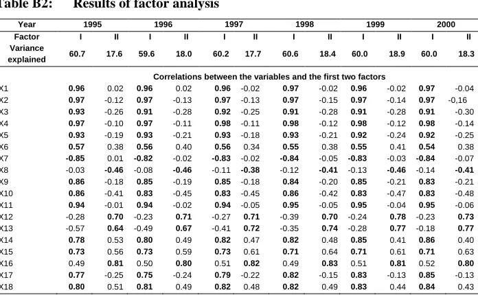
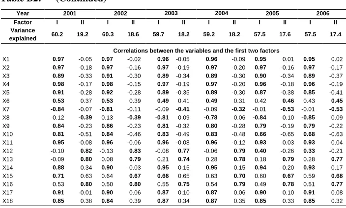
As a preliminary examination of the indexes considered showed the presence of correlations that rendered them unsuitable for use in a regression model, they have been synthesised by means of factor analysis. The results of this analysis are set out in Appendix B (Table B2). The factor structure, which was identified using the varimax orthogonal rotation of the SAS System software ver. 9.2, was found to be very stable in time, and to have a considerable capacity for synthesis. The first two factors, according to the usual criteria of factor choice, lend themselves to immediate interpretation. The high and positive correlation coefficients between the first factor and all of the manifest variables of economic nature suggest that this factor is a complex index of the economic structure, while the close correlations of the second factor with the remaining indexes suggest that we should identify this index as a complex index of the demographic structure.
Taking these considerations into account, we decided to analyse the migratory flows between the 20 Italian regions in the period from 1995 to 2006 using the following time series cross-sectional spatial interaction model:
+ = S;2006 S;1995 I;2006 I;1995 S;2006 S;1995 I;2006 I;1995 S;2006 S;1995 I;2006 I;1995 S;2006 S;1995 I;2006 I;1995 .. .. .. .. .. .. .. .. .. .. .. .. .. .. .. .. .. .. .. .. .. .. .. .. .. .. .. .. .. .. .. .. ε ε ε ε β β β β X 0 0 0 X X 0 0 0 X F F F F (3)
where I indicates the group of Italians and S indicates the group of resident foreigners, while FI;t and FS;t (for t=1995,..,2006) are the vectors (380x1) containing the logarithm of the annual frequency of the changes of residence of the Italians (I), and the resident foreigners (S), from the i-th region to the j-th region (lg(fij;t)).
XI;t and XS;t (for t=1995,..,2006) are matrices, with each of them containing for each year the whole set of the covariates considered for the Italians and the foreign residents, respectively, and in the following order:
The logarithmic of the size of the resident population in the origin-regions of flows (lg(Pi;t)) and destination-regions of flows (lg(Pj;t));
The logarithmic of the geographic distance between two generic regions (lg(dij;t)); The first two factors extracted from the 18 variables considered in the origin and the destination regions of flows; i.e., F1i;t, F1j;t for the first factor (economic) and F2i;t, F2j;t for the second factor (demographic);
The eigenvectors spatial filtering, in particular, Eko for the autocorrelation at the origin and Ekd for the autocorrelation at the destination (see Table B1).
βI;t and βS;t (for t=1995,..,2006) are vectors containing the parameters of the model. εg;t (for g=I; S) is the usual residual variable.
The annual resident population (Pi;t and Pj;t) was calculated as the geometric average of the population at the beginning and at the end of each year. The distances (dij) between the regions were instead calculated by considering the Euclidean distance between the demographic barycentres of each region.8
Finally, by means of the Chow test (Chow 1960), both the temporal stability of the model parameters and their diversity in the two groups were tested.
It should be noted that, given the nature of the dependent variable (count data), the linear regression model was chosen instead of the Poisson regression model, in part because a preliminary analysis of the data showed the widespread presence of the well-known problem of overdispersion (see TableB3).
8 The pairs of co-ordinates identifying each regional demographic barycentre were determined by calculating
A second reason for this choice was that our investigation was intended to be explanatory, not predictive; i.e., our only goal was to identify the covariates influencing migration flows. A third reason was that the mean flows (see Table B3) take values such that—as Baltagi (2011), Lejenne (2010), and Hayter (2012) reported—the Poisson random variable can be well approximated by the normal variable. Therefore, the parameter estimates of the two models, as the authors have tested, are analogous. Fourth, the linear regression model makes it easier to interpret the results. Finally, the use of this model is in full accordance with the literature; see, for example, Black (1992); Clark, Hatton, and Williamson (2007); Egger (2005); Fischer, Reismann, and Scherngell (2006); Fischer and Griffith (2008b); Lewer and Van den Berg (2008); Griffith (2009); Kim and Koen (2010); Mayda (2010); and Ludo (2012).
3. Results
Before discussing the results of our analysis, we should point out that, mainly for the group of resident foreigners, the F matrix of flows had a number of zero entries in some years.
In these cases, for estimation purposes, it is usual to add a constant 0<α≤1 to all the entries of F. However, as Flowerdew and Aitkin (1982) noted, different values of α may have different effects on the parameter estimates of the model.
Thus, the following strategy was used. Model (3) was estimated setting the following values for α: 0.1, 0.3, 0.5, 0.7, and 1. Then the constant value was chosen using the log likelihood, Akaike, and Schwarz criteria.
All of the criteria indicated that α=1 should be assigned as the optimal value (see Table B4). This choice is in line with several studies which have recommended the use of the lowest possible non-zero count in this situation (see, for instance, Van Bergijk and Steven 2010).
Furthermore, we assumed that, contrary to the results of Flowerdew and Aitkin (1982), the parameter estimates of model (3) undergo negligible changes for different values of α (results not shown, but available upon request).
Second, the index of determination (corrected R2) was found to have been very high (about 98%). As this index could be misleading because of the presence of good leverage flows (good outliers), the potential outlier flows were identified using Cook’s d statistic, and the model was re-estimated by dropping them from the data set.
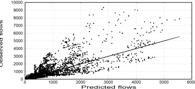
A further test was conducted in order to assess the predictive ability of the model. This was not, however, the goal of the paper. In Figure A2 in the appendix, the scatterplots of the observed versus the fitted flows for the two groups of residents are shown. We can see that there was a slight underestimation of large migration flows.
Finally, the tests of White, Kolmogorov-Smirnov, and the Moran Index showed that the regression residuals were, respectively, homoscedastic, normally distributed, and spatially uncorrelated at the origin and the destination of flows.
When we looked at the results on the migratory movements of the Italians, we could see that for the entire time period of 1995-2006, the estimates of the constant and the parameters associated with the population size of the regions, as well as the parameter relative to the distance, were always highly significant. The sign of the parameter of the latter variable was negative and consistent with expectations.
The estimates of the parameters associated with the economic factor in the regions of origin and in the destination regions of flows (F1i and F1j respectively) were also always highly significant. According to the signs, this factor was a push determinant in the regions of origin and a pull determinant in the destination regions of flows, while in the absolute values no noticeable predominant effect like a push or pull determinant was evident.
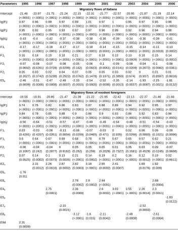
Table 1: Estimates of log spatial interaction model (3)
F-Fisher related to the model 2066.23 p-value=<0.0001
R2
corrected 0.9815
White Test of heteroskedasticity 6.67 p-value=0.01
Kolmogorov-Smirnov test of normality 0.011 p-value=0.013
Moran Index of autocorrelation at the origin 0.313 p-value=0.08
Table 1: (Continued)
Parameters 1995 1996 1997 1998 1999 2000 2001 2002 2003 2004 2005 2006
Migratory flows of Italians
Intercept -21.46 -20.97 -21.75 -21.24 -22.15 -22.31 -21.77 -22.57 -20.95 -21.87 -21.19 -22.14
(<.0001) (<.0001) (<.0001) (<.0001) (<.0001) (<.0001) (<.0001) (<.0001) (<.0001) (<.0001) (<.0001) (<.0001)
lg(Pi) 0.97 0.96 0.99 0.97 0.99 1.01 0.97 1 0.95 0.97 0.95 0.98
(<.0001) (<.0001) (<.0001) (<.0001) (<.0001) (<.0001) (<.0001) (<.0001) (<.0001) (<.0001) (<.0001) (<.0001)
lg(Pj) 0.95 0.92 0.95 0.93 0.97 0.97 0.96 0.99 0.92 0.96 0.94 0.98
(<.0001) (<.0001) (<.0001) (<.0001) (<.0001) (<.0001) (<.0001) (<.0001) (<.0001) (<.0001) (<.0001) (<.0001)
lg(dij) -0.43 -0.4 -0.42 -0.37 -0.38 -0.38 -0.36 -0.39 -0.34 -0.36 -0.39 -0.41
(<.0001) (<.0001) (<.0001) (<.0001) (<.0001) (<.0001) (<.0001) (<.0001) (<.0001) (<.0001) (<.0001) (<.0001)
F1i -0.17 -0.17 -0.18 -0.17 -0.17 -0.18 -0.14 -0.15 -0.15 -0.14 -0.11 -0.13
(<.0001) (<.0001) (<.0001) (<.0001) (<.0001) (<.0001) (0.0001) (<.0001) (<.0001) (<.0001) (0.0018) (0.0002)
F1j 0.16 0.18 0.15 0.18 0.21 0.17 0.18 0.15 0.13 0.18 0.15 0.14
(<.0001) (<.0001) (0.0001) (<.0001) (<.0001) (<.0001) (<.0001) (<.0001) (0.0009) (<.0001) (<.0001) (0.0002)
F2i -0.07 -0.08 -0.07 -0.08 -0.05 -0.06 -0.1 -0.09 -0.08 -0.04 -0.1 -0.08
(0.0692) (0.0261) (0.0728) (0.0299) (0.162) (0.0923) (0.0061) (0.0141) (0.0209) (0.2672) (0.0082) (0.0361)
F2j 0.05 0.03 0.02 0.04 0.07 0.05 0.05 0.03 0.02 0 0.01 0.01
(0.2027) (0.3742) (0.5238) (0.2922) (0.0762) (0.1478) (0.1971) (0.3859) (0.674) (0.937) (0.8597) (0.8016)
E5d -2.46 -2.51 -2.47 -2.49 -2.33 -2.54 -2.52 -2.35 -2.14 -1.93 -2.25 -1.81
(0.0009) (0.0006) (0.0008) (0.0007) (0.0015) (0.0005) (0.0006) (0.0013) (0.0037) (0.0087) (0.0021) (0.0132)
Migratory flows of resident foreigners
Intercept -19.56 -18.91 -20.85 -21.47 -21.39 -21.22 -21.95 -22.42 -22.13 -22.37 -21.46 -21.66
(<.0001) (<.0001) (<.0001) (<.0001) (<.0001) (<.0001) (<.0001) (<.0001) (<.0001) (<.0001) (<.0001) (<.0001)
lg(Pi) 0.74 0.76 0.82 0.86 0.83 0.87 0.88 0.89 0.94 0.92 0.95 0.97
(<.0001) (<.0001) (<.0001) (<.0001) (<.0001) (<.0001) (<.0001) (<.0001) (<.0001) (<.0001) (<.0001) (<.0001)
lg(Pj) 0.84 0.78 0.85 0.88 0.9 0.86 0.9 0.93 0.86 0.92 0.83 0.96
(<.0001) (<.0001) (<.0001) (<.0001) (<.0001) (<.0001) (<.0001) (<.0001) (<.0001) (<.0001) (<.0001) (<.0001)
lg(dij) -0.56 -0.64 -0.51 -0.57 -0.47 -0.49 -0.49 -0.54 -0.48 -0.51 -0.54 -0.43
(<.0001) (<.0001) (<.0001) (<.0001) (<.0001) (<.0001) (<.0001) (<.0001) (<.0001) (<.0001) (<.0001) (<.0001)
F1i 0.03 -0.03 -0.08 -0.13 -0.08 -0.07 -0.03 0 0.02 0.06 0.06 -0.09
(0.4291) (0.4207) (0.0351) (0.0004) (0.0209) (0.0465) (0.471) (0.935) (0.5266) (0.0893) (0.1021) (0.0096)
F1j 0.6 0.64 0.67 0.69 0.68 0.78 0.79 0.67 0.65 0.57 0.62 0.21
(<.0001) (<.0001) (<.0001) (<.0001) (<.0001) (<.0001) (<.0001) (<.0001) (<.0001) (<.0001) (<.0001) (<.0001)
F2i -0.06 -0.04 -0.04 0 0.05 0.05 0.05 0.01 0.05 0.03 0.09 -0.07
(0.1087) (0.242) (0.2877) (0.9162) (0.262) (0.259) (0.2029) (0.7327) (0.1581) (0.4529) (0.0245) (0.0668)
F2j 0.07 0.14 0.1 0.13 0.21 0.14 0.19 0.2 0.16 0.12 0.19 0.02
(0.0525) (0.0002) (0.0073) (0.0005) (<.0001) (0.0002) (<.0001) (<.0001) (<.0001) (0.0012) (<.0001) (0.6611)
E2o 2.31 2.26 2.67 2.62 3.18 2.65 2.41 1.69 1.92
(0.0012) (0.0016) (0.0002) (0.0003) (<.0001) (0.0002) (0.0007) (0.0176) (0.009)
E6o -1.76
(0.01)
E8o 2.78 2.8 2.94 2.68
(0.0002) (0.0002) (<.0001) (0.0004)
E4d 2.75 2.36 2.6 3.03 3.55 2.26 2.3
(0.0001) (0.0009) (0.0002) (<.0001) (<.0001) (0.0014) (0.0011)
E5d -1.83
(0.0122)
E7d -2.15 -2.52
(0.0021) (0.0003)
E8d -3.12 -1.8 -2.11 -2.48 -2.61
(<.0001) (0.015) (0.0042) (0.0008) (0.0004)
E9d 2.31
(0.0009)
When we looked at the demographic factor of the places of origin (F2i) and of the places of destination (F2j), the estimates of the associated parameters were found to have been non-significant for some years of the period considered. But the constancy of sign and the weak temporal variability led us to conclude that the demographic characteristics of the Italian regions played a role, albeit a minor one, in determining the migratory movements of Italians, and was more significant as an expulsive than as an attractive force.
Moreover, the estimates of the coefficients of all of these variables exhibited— from year to year and between the end and the beginning of the period—values that were not significantly different, which highlights the presence of a constant temporal effect on the migratory movements of the Italian residents9.
In sum, it appears that the regional migration flows of the Italians were affected by all of the variables considered: the size of the populations, the geographical distance, the economic conditions, and, to a lesser extent, the demographic conditions of the regions.
Finally, the Italians’ migratory flows were influenced by some degree of spatial autocorrelation.
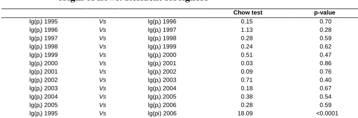
When we looked at migrations between Italian regions by the resident foreigners, we once again found that the classic determinants of the gravity model (size of populations and geographical distance between regions) were always highly significant, but that, unlike among the Italians, there was an increasing and significant effect over time of the population size of the regions of destination, and especially of origin (Tables B5 and B6).
Among the remaining variables, the economic and demographic factors of the regions of the destination of flows (F1j and F2j respectively) certainly acted as pull determinants (the estimates of the associated parameters were always significant except for the demographic factor in 2006). The findings indicated, however, that the demographic factor of the regions of origin (F2i) was not a determinant of the outflows of the resident foreigners, as the parameter estimates over the time period considered were almost never significant, and their signs did not persist. The influence of the economic conditions of the regions of destination of flows increased until 2001, and then decreased, especially in the last year considered; while the influence of the demographic conditions of the same regions increased until 1999, and then stabilised until 2005 (Tables B7 and B8).
Regarding the economic factor of the regions of origin (F1i), we found that it significantly influenced—albeit without a varying temporal effect (Table B9), and only
to a small extent—the migratory movements of the resident foreigners only in the years 1997-2000 and 2006.
Finally, the migratory flows of the resident foreigners also showed a certain level of spatial autocorrelation, but in this case the sign was often positive.
When considering the mobility patterns of the Italians and the resident foreigners, it should be noted that, among the classic determinants of the spatial interaction model, distance hadthe same effect on the mobility of the two groups, with the exception of the years 1996 and 1998 (Table B10). The population size of the regions of origin had a greater effect on the mobility of Italians than on the mobility of resident foreigners, which was statistically significant in the period 1995 to 2000 and in 2002 (Table B11). In addition, the effect of the population size of the regions of destination was higher for Italians than for resident foreigners, which in this case was statistically significant only in the years 1995-1997, 2000, and 2005 (Table B12).
The economic and demographic factors acted in rather different ways in the two cases analysed. While in the destination regions they constituted pull factors, albeit to different degrees, for the migratory movements of both the Italians and the resident foreigners, the demographic situation of the sending regions was a push factor only for the mobility of the Italians. It also has to be stressed that the economic conditions of the sending regions had a much greater effect on the Italians than on the resident foreigners (the difference was statistically significant in the years for which a comparison is meaningful, except in 1998 and 2006, Table B13), while better economic conditions in the destination regions had a greater effect on the resident foreigners than on the Italians (the difference was statistically significant except in 2006, Table B14).
In addition, the demographic characteristics of the destination regions had a greater effect on the migratory flows of the resident foreigners than on the mobility of the Italians, and the difference was statistically significant over most of the period (Table B15).
Regardless of the group considered, however, the findings indicated that the demographic conditions of regions—when explicative of internal migration—always played a less important role than the economic conditions in explaining migration (Tables B16-B18).
4. Conclusions
Our analysis, conducted by means of a particular gravity model which considers, in addition to the classic determinants, the effects exerted by a set of economic and demographic variables and those attributable to a possible spatial autocorrelation of flows, points to the complexity of internal migration in Italy from 1995 to 2006. It clearly shows the differences in the determinants of mobility among the Italians and the resident foreigners studied, and an explicative frame in evolution for the resident foreigners.
In the period considered, the population sizes of the regions and the distances between them were important determinants of migratory flows for both the Italians and the foreigners. In particular, the population sizes of the regions, both of origin and destination, were more important for the Italians than for the resident foreigners. Thus, different mobility patterns for the two groups were revealed: the Italians moved mainly towards more populated regions, while the resident foreigners made more varied choices, although the tendency to move to more densely populated territories increased over time. However, both the Italians and the resident foreigners were equally discouraged from migrating over longer distances.
The evidence of different mobility patterns is strengthened by the different effects found for the two factors which synthesise the economic and demographic conditions of a region. Among the Italians, moves were highly influenced by economic conditions: they were pushed to relocate by economic difficulties and were attracted by better economic conditions or opportunities. For the Italians, demographic factors were influential, but were not predominant. By contrast, when the foreigners moved out of their region of residence, they were not pushed by either the demographic situation, or, except for a limited period of time, the economic conditions. However, both the economic and the demographic conditions attracted them to other regions, with the extent of these influences changing over time. In particular, the effect of demographic conditions showed an overall tendency to increase. It should also be emphasised that economic conditions had a greater effect than the demographic variables on the foreign residents, and that economic conditions had a larger effect in general on the foreign residents than on the Italians.
References
Attanasio, O. and Padoa-Schioppa, F. (1991). Regional inequalities, migration and labour mismatch in Italy, 1960-1986. In: Padoa-Schioppa, F. (ed.). Mismatch and Labour Mobility. Cambridge: Cambridge University Press: 237-324.
Arru, A. and Ramella, F. (2003). Introduzione. In: Arru, A. and Ramella, F. (eds.). L’Italia delle migrazioni interne: Donne, uomini, mobilità in età moderna e contemporanea. Roma: Donzelli: IX-XX.
Baltagi, H.B. (2011). Econometrics. 5th edition. Berlin/Heidelberg: Springer. doi:10.1007/978-3-642-20059-5.
Black, W.R. (1992). Network autocorrelation in transport network and flow system. Geographical Analysis 24(3): 207-222. doi:10.1111/j.1538-4632.1992.tb 00262.x.
Bodvarsson, Ö.B. and Van den Berg, H. (2009). The Economics of Immigration: Theory and Policy. Berlin/Heidelberg: Springer.
Bonifazi, C. (1999). Introduzione. In: Bonifazi, C. (ed.). Mezzogiorno e migrazioni interne, Monografie n.10. Roma: Consiglio Nazionale delle Ricerche, Istituto di Ricerche sulla Popolazione: 1-16.
Bonifazi, C. and Heins, F. (2000). Long-term trends of internal migration in Italy. International Journal of Population Geography 6: 111-131. doi:10.1002/(SICI)1099-1220(200003/04)6:2<111::AID-IJPG172>3.0.CO;2-L.
Casacchia, O. and Strozza, S. (2002). Le migrazioni interne e internazionali in Italia dall’Unità ad oggi: un quadro di sintesi. In: Di Comite, L. and Paterno, A. (eds). Quelli di fuori. Dall’emigrazione all’immigrazione: Il caso italiano. Milano: Franco Angeli: 50-88.
Chow, G.C. (1960). Tests of equality between sets of coefficients in two linear regressions. Econometrica 28(3): 591–605. doi:10.2307/1910133.
Chun, Y. (2008). Modeling network autocorrelation within migration flows by eigenvector spatial filtering. Journal of Geographical System 10: 317-344. doi:10.1007/s10109-008-0068-2.
Clark, T., Hatton, T.J., and Williamson, G.J. (2007). Explaining U.S. immigration, 1971-1998. The Review of Economics and Statistics 89(2): 359-373. doi:10.1162/rest.89.2.359.
Cuffaro, M. and Giaimo, R. (2005). Convergenza economica e mobilità territoriale. Rivista Italiana di Economia Demografia e Statistica LIX(1-2): 61-78.
De Santis, G. (2010). Mobilità a corto e a lungo raggio e pendolarismo della popolazione italiana. In: Livi Bacci, M. (ed.). Demografia del capitale umano. Bologna: Il Mulino: 123-138.
Deshingkar, P. and Grimm, S. (2005). International migration and development: A global perspective. Geneva: International Organization for Migration (IOM Migration Research Series; 19).
Egger, P. (2005). Alternative techniques for estimation of cross-section gravity models. Review of International Economics 13(5): 881-891. doi:10.1111/ j.1467-9396.2005.00542.x.
Etzo, I. (2011). The determinants of the recent interregional migration flows in Italy: A panel data analysis. Journal of Regional Sciences 51(5): 948-966. doi:10.1111/j.1467-9787.2011.00730.x.
Evenett, S.J. and Keller, W. (2002). On the theories explaining the success of the gravity equation. Journal of Political Economy 110: 281-316. doi:10.1086/338746.
Fachin, S. (2007). Long-run trends in internal migration in Italy: A study in panel cointegration with dependent units. Journal of Applied Econometrics 22: 401-428. doi:10.1002/jae.907.
Faini, R., Galli, G., Gennari, P., and Rossi, F. (1997). An empirical puzzle: Falling migration and growing unemployment differentials among Italian regions. European Economic Review 41: 571-579. doi:10.1016/S0014-2921(97)00023-8.
Fischer, M.M. and Griffith, D.A. (2008a). Modeling spatial autocorrelation in spatial interaction data: An application to patent citation in the European union. Journal of Regional Science 48(5): 969-989. doi:10.1111/j.1467-9787.2008.00572.x.
Fischer, M., Reismann, M., and Scherngell, T. (2006). From conventional to spatial econometrics models of spatial interactions. Paper presented at the International Workshop on Spatial Econometrics and Statistics, Rome, Italy, 25-27 May 2005. Flowerdew, R. and Aitkin, M. (1982). A method of fitting the gravity model based on the Poisson distribution. Journal of Regional Science 22(2): 191-202. doi:10.1111/j.1467-9787.1982.tb00744.x.
Forcellati, L. and Strozza, S. (2006). Modelli insediativi delle comunità straniere in Italia: un quadro di sintesi. Rivista Italiana di Economia Demografia e Statistica LX(1-2): 127-150.
Griffith, D.A. (2003). Spatial autocorrelation and spatial filtering. Berlin/Heidelberg: Springer. doi:10.1007/978-3-540-24806-4.
Griffith, D.A. (2008). Spatial filtering-based contributions to a critique of geographically weighted regression (GWR). Environment & Planning A40(11): 2751-2769. doi:10.1068/a38218.
Griffith, D.A. (2009). Modeling spatial autocorrelation in spatial interaction data: Empirical evidence from 2002 Germany journey-to-work flows. Journal of Geographical System 11: 117-140. doi.org/10.1007/s10109-009-0082-z.
Harris, J.R. and Todaro, M.P. (1970). Migration, unemployment and development: A two sector analysis. American Economic Review 60(1): 126-142.
Hayter, A. (2012). Probability and statistics for engineers and scientist. Boston: Brooks/Cole.
Hugo, G. (1981). Village-community ties, village norms, and ethnic and social networks: A review of evidence from the third world. In: DeJond, G. and Gardner, R. (eds.). Migration decision making: Multidisciplinary approaches to microlevel studies in developed and developing countries. New York: Pergamon Press: 186-224.
Isard, W. (1998). Gravity and spatial interaction models. In: Isard, W., Azis, I.J., Drennan, M.P., Miller, R.E., Saltzman, S., and Thorbecke, E. (eds.). Methods of interregional and regional analysis. Cambridge: Ashgate Publishing Limited: 243-280.
ISTAT (2010). La popolazione straniera residente in Italia al 1° gennaio 2010. Roma: ISTAT. (Statistiche in breve).
Karemera, D., Iwuagwu Oguledo, V., and Davis, B. (2000). A gravity model analysis of international migration to North America. Applied Economics 32: 1745-1755. doi:10.1080/000368400421093.
Kim, K. and Koen, E.J. (2010). Determinants of international migration flows to and from industrialized countries: A panel data approach beyond gravity. International Migration Review 44(4): 899-932. doi:10.1111/j.1747-7379.2010. 00830.x.
Lejenne, M. (2010). Statistique la théorie e ses application. Paris: Springer.
LeSage, J.P. (2004). Spatial regression models. In: Altman, M., Gill, J., and McDonald, M. (eds). Numerical Issues in Statistical Computing for the Social Scientist. New York: John Wiley & Sons, 199- 218.
LeSage, J.P. and Pace, R. (2007). Spatial econometric modelling of the origin-destination flows. Journal of Regional Science 48: 941-967. doi:10.1111/ j.1467-9787.2008.00573.x.
Lewer, J.J. and Van den Berg, H. (2008). A gravity model of immigration. Economic Letters 99: 164-167. doi:10.1016/j.econlet.2007.06.019.
Lewis, W.A. (1954). Economic development without unlimited supplies of labor. The Manchester School of Economic and Social Studies 22: 139-191. doi:10.1111/j.1467-9957.1954.tb00021.x.
Livi Bacci, M. (2010). Introduzione. In: Livi Bacci, M. (ed.). Demografia del capitale umano. Bologna: Il Mulino: 9-27.
Ludo, P. (2012). Gravity and spatial structure: The case of interstate migration in Mexico. Journal of Regional Science 52(5): 819-856. doi:10.1111/j.1467-9787. 2012.00770.x.
Massey, D.S., Arango, J., Hugo, G., Kouaouci, A., Pellegrino, A., and Taylor, J.E. (1993). Theories of international migration: A review and appraisal. Population and Development Review 19(3): 431-466. doi:10.2307/2938462.
Massey, R. and Garcia Espana, F. (1987). The social process of international migration. Science 237: 733-738. doi:10.1126/science.237.4816.733.
Mayda, A.M. (2010). International migration: A panel data analysis of the determinant of bilateral flows. Journal of Population Economics 23: 1249-1274. doi:10.1007/s00148-009-0251-x.
Mocetti, S. and Porello, C. (2010a). La mobilità del lavoro in Italia: nuove evidenze sulle dinamiche migratorie. Questioni di Economia e Finanza no. 61. Roma: Banca d’Italia.
Mocetti, S. and Porello, C. (2010b). How does immigration affect native internal mobility? New evidence from Italy. Temi di discussione no. 748. Rome: Banca d’Italia.
Patuelli, R., Schanne, N., Griffith, D.A., and Nijkamp, P. (2012). Persistence of regional unemployment: Application of a spatial filtering approach to local labor markets in Germany. Journal of Regional Science 52(2): 300-323. doi:10.1111/j.1467-9787.2012.00759.x.
Piras, R. (2010). Internal migration across Italian regions: Macroeconomic determinants and accommodating potentials for a dualistic economy. Nota di lavoro no. 115. Milano: Fondazione Enrico Mattei.
Piras, R. and Melis, S. (2007). Evoluzioni e tendenze delle migrazioni interne. Economia Italiana 2: 437-461.
Porojan, A. (2001). Trade flows and spatial effects: The gravity model revisited. Open Economies Review 12(3): 265-280. doi:10.1023/A:1011129422190.
Pugliese, E. (2006). L’Italia tra migrazioni internazionali e migrazioni interne. Bologna: Il Mulino.
Ranis, G. and Fei, J.C.H. (1961). A theory of economic development. American Economic Review 51(4): 533-565.
Salvatore, D. (1977). An econometric analysis of internal migration in Italy. Journal of Regional Science 17(3): 395-408. doi:10.1111/j.1467-9787.1977.tb00510.x.
Sen, A.K. and Smith, T.E. (1995). Gravity models of spatial interaction behavior. London: Springer. doi:10.1007/978-3-642-79880-1.
Van Bergeijk, P.A.G. and Steven, B. (2010). The gravity model in international trade: Advanced and application. Cambridge: Cambridge University Press. doi:10.1017/CBO9780511762109.
Appendix A
Socio-economic and demographic variables
X1) Employment rate = Employed resident population / Total population resident in the region.
X2) Added value per capita = Regional added value / Total population resident in the region.
X3) Added value per person employed = Regional added value / Employed resident population.
X4) GDP per capita = Regional GDP / Population resident in the region.
X5) GDP per person employed = Regional GDP / Employed resident population. X6) % of employed in industry = Share of population resident in the region employed
in industry.
X7) % of employed in agriculture = Share of population resident in the region employed in agriculture.
X8) % of employed in other activities = Share of population resident in the region employed in activities other than industry and agriculture.
X9) Consumption per capita = Resident population consumption / Total population resident in the region.
X10) Income per capita = Resident population income / Total population resident in the region.
X11) Units of labour per inhabitant = Number of regional labour units / Total population resident in the region.
X12) Size of unit of labour = Number of employed in the region / Number of regional labour units.
X13) Age dependency ratio = Regional resident population aged 65+ / Regional resident population aged 15-64.
X14) Index of turnover in the active population = Regional resident population aged 15-19 / Regional resident population aged 60-64.
X15) Portion of persons aged 65 and over = Regional resident population aged 65+/ Regional resident population.
X16) Old-age dependency ratio = Regional resident population aged 65+ / Regional resident population aged 15-64.
X17) % of resident foreigners to total population = Number of foreigners resident in the region / Total population resident in the region.
Figure A2: Scatterplots of the linear regression model for Italians and resident foreigners
Italians
RMSE=721.6
Resident foreigners
Appendix B
Table B1: Selected eigenvectors
Italians Resident foreigners
Year Origin autocorr. Destin. autocorr. Origin autocorr. Destin. autocorr.
1995 - E5d E6o E9d
1996 - E5d E2o E4d
1997 - E5d E2o -
1998 - E5d E2o E7d
1999 - E5d E2o; E8o E4d; E8d
2000 - E5d E2o; E8o E8d
2001 - E5d E2o; E8o E4d; E8d
2002 - E5d E2o E4d
2003 - E5d - E4d; E8d
2004 - E5d E2o E4d; E7d
2005 - E5d E2o; E8o E4d; E8d
2006 - E5d E5o -
Table B2: Results of factor analysis
Year 1995 1996 1997 1998 1999 2000
Factor I II I II I II I II I II I II
Variance
explained 60.7 17.6 59.6 18.0 60.2 17.7 60.6 18.4 60.0 18.9 60.0 18.3
Correlations between the variables and the first two factors
X1 0.96 0.02 0.96 0.02 0.96 -0.02 0.97 -0.02 0.96 -0.02 0.97 -0.04 X2 0.97 -0.12 0.97 -0.13 0.97 -0.13 0.97 -0.15 0.97 -0.14 0.97 -0,16 X3 0.93 -0.26 0.91 -0.28 0.92 -0.25 0.91 -0.28 0.91 -0.28 0.91 -0.30 X4 0.97 -0.10 0.97 -0.11 0.98 -0.11 0.98 -0.12 0.98 -0.12 0.98 -0.14 X5 0.93 -0.19 0.93 -0.21 0.93 -0.18 0.93 -0.21 0.92 -0.24 0.92 -0.25 X6 0.57 0.38 0.56 0.40 0.56 0.34 0.55 0.38 0.55 0.41 0.54 0.38 X7 -0.85 0.01 -0.82 -0.02 -0.83 -0.02 -0.84 -0.05 -0.83 -0.03 -0.84 -0.07
X8 -0.03 -0.46 -0.08 -0.46 -0.11 -0.38 -0.12 -0.41 -0.13 -0.46 -0.14 -0.41
X9 0.86 -0.18 0.85 -0.19 0.85 -0.18 0.84 -0.20 0.85 -0.21 0.83 -0.21 X10 0.86 -0.41 0.83 -0.45 0.83 -0.45 0.86 -0.42 0.83 -0.47 0.83 -0.48 X11 0.94 -0.01 0.94 -0.02 0.94 -0.05 0.95 -0.05 0.95 -0.04 0.95 -0.06
X12 -0.28 0.70 -0.23 0.71 -0.27 0.71 -0.39 0.70 -0.24 0.78 -0.23 0.73
X13 -0.57 0.64 -0.49 0.67 -0.41 0.72 -0.35 0.74 -0.28 0.77 -0.18 0.77
X14 0.78 0.53 0.80 0.49 0.82 0.47 0.82 0.48 0.85 0.41 0.86 0.40 X15 0.73 0.56 0.73 0.59 0.73 0.61 0.71 0.64 0.71 0.61 0.71 0.63
X16 0.49 0.81 0.50 0.80 0.51 0.82 0.49 0.83 0.51 0.81 0.52 0.80
Table B2: (Continued)
Year 2001 2002 2003 2004 2005 2006
Factor I II I II I II I II I II I II
Variance
explained 60.2 19.2 60.3 18.6 59.7 18.2 59.2 18.2 57.5 17.6 57.5 17.4
Correlations between the variables and the first two factors
X1 0.97 -0.05 0.97 -0.02 0.96 -0.05 0.96 -0.09 0.95 0.01 0.95 0.02 X2 0.97 -0.18 0.97 -0.16 0.97 -0.19 0.97 -0.20 0.97 -0.16 0.97 -0.17 X3 0.89 -0.33 0.91 -0.30 0.89 -0.34 0.89 -0.30 0.90 -0.34 0.89 -0.37 X4 0.98 -0.17 0.98 -0.15 0.97 -0.19 0.97 -0.20 0.96 -0.18 0.96 -0.19 X5 0.91 -0.28 0.92 -0.28 0.89 -0.35 0.89 -0.30 0.87 -0.38 0.85 -0.41 X6 0.53 0.37 0.53 0.39 0.49 0.41 0.49 0.31 0.42 0.46 0.43 0.45
X7 -0.84 -0.07 -0.81 -0.11 -0.09 -0.41 -0.09 -0.32 -0.01 -0.53 -0.01 -0.53
X8 -0.12 -0.39 -0.13 -0.39 -0.81 -0.09 -0.78 -0.06 -0.84 0.10 -0.85 0.09
X9 0.84 -0.23 0.86 -0.23 0.81 -0.32 0.80 -0.28 0.79 -0.19 0.79 -0.22 X10 0.81 -0.51 0.84 -0.46 0.83 -0.49 0.83 -0.48 0.66 -0.65 0.68 -0.63 X11 0.95 -0.08 0.96 -0.06 0.96 -0.08 0.96 -0.12 0.93 0.03 0.93 0.04
X12 -0.10 0.82 -0.13 0.83 -0.08 0.77 -0.06 0.79 0.40 -0.26 0.33 -0.21
X13 -0.09 0.80 0.08 0.79 0.21 0.74 0.28 0.78 0.18 0.79 0.28 0.77
X14 0.88 0.34 0.90 -0.03 0.95 0.15 0.95 0.15 0.94 -0.20 0.93 -0.17 X15 0.71 0.63 0.64 0.67 0.66 0.65 0.63 0.70 0.60 0.67 0.59 0.68
X16 0.53 0.80 0.50 0.80 0.55 0.75 0.54 0.79 0.49 0.78 0.51 0.77
X17 0.91 -0.01 0.90 0.06 0.87 0.10 0.87 0.06 0.90 0.10 0.91 0.08 X18 0.85 0.38 0.84 0.39 0.87 0.34 0.87 0.35 0.85 0.33 0.85 0.32
Table B3: Descriptive statistics of the flow matrices
Italians Resident foreigners
Year Mean Variance Mean Variance
1995 722.0474 1143974.2194 34.0105 3675.6252
1996 743.7105 1290312.2590 35.5105 4098.8205
1997 762.4842 1310048.9206 44.9526 6561.1904
1998 793.8105 1455950.1962 59.8026 13318.0058
1999 821.8342 1621330.4131 60.4658 12953.9276
2000 869.5158 1781113.9602 74.9000 20226.0269
2001 762.5737 1411707.4431 78.6474 22861.1260
2002 800.1342 1499521.0030 83.9868 26260.5196
2003 772.5632 1304630.7058 82.8789 24026.9141
2004 775.4474 1335239.0605 106.5211 36824.2608
2005 757.0579 1266515.9017 113.6237 44311.3488
2006 761.9684 1296409.5557 86.9568 16290.7347
Table B4: Selection criteria for different α values
α values Log-likelihood Akaike criterion Schwarz criterion
0.1 -10971.02 24075.70 22410.04
0.3 -9918.645 21970.96 20305.29
0.5 -9527.813 21189.29 19523.63
0.7 -9320.830 20775.33 19109.66
Table B5: Temporal comparison of the resident population parameter of the origin of flows. Resident foreigners
Chow test p-value
lg(pi) 1995 Vs lg(pi) 1996 0.15 0.70
lg(pi) 1996 Vs lg(pi) 1997 1.13 0.28
lg(pi) 1997 Vs lg(pi) 1998 0.28 0.59
lg(pi) 1998 Vs lg(pi) 1999 0.24 0.62
lg(pi) 1999 Vs lg(pi) 2000 0.51 0.47
lg(pi) 2000 Vs lg(pi) 2001 0.03 0.86
lg(pi) 2001 Vs lg(pi) 2002 0.09 0.76
lg(pi) 2002 Vs lg(pi) 2003 0.71 0.40
lg(pi) 2003 Vs lg(pi) 2004 0.18 0.67
lg(pi) 2004 Vs lg(pi) 2005 0.38 0.54
lg(pi) 2005 Vs lg(pi) 2006 0.28 0.59
lg(pi) 1995 Vs lg(pi) 2006 18.09 <0.0001
Table B6: Temporal comparison of the resident population parameter of the
destination of flows. Resident foreigners
Chow test p-value
lg(pj) 1995 Vs lg(pj) 1996 1.25 0.26
lg(pj) 1996 Vs lg(pj) 1997 2.32 0.12
lg(pj) 1997 Vs lg(pj) 1998 0.47 0.49
lg(pj) 1998 Vs lg(pj) 1999 0.10 0.74
lg(pj) 1999 Vs lg(pj) 2000 0.56 0.45
lg(pj) 2000 Vs lg(pj) 2001 0.66 0.42
lg(pj) 2001 Vs lg(pj) 2002 0.29 0.59
lg(pj) 2002 Vs lg(pj) 2003 1.93 0.16
lg(pj) 2003 Vs lg(pj) 2004 1.62 0.20
lg(pj) 2004 Vs lg(pj) 2005 3.32 0.07
lg(pj) 2005 Vs lg(pj) 2006 6.00 0.01
lg(pj) 1995 Vs lg(pj) 2006 5.96 0.014
Table B7: Temporal comparison of parameters related to the economic factor
in the destination regions of flows. Resident foreigners
Chow test p-value
F1J 1995 Vs F1J 1996 0.51 0.47
F1J 1996 Vs F1J 1997 0.46 0.50
F1J 1997 Vs F1J 1998 0.11 0.74
F1J 1998 Vs F1J 1999 0.03 0.86
F1J 1999 Vs F1J 2000 3.5 0.061
F1J 2001 Vs F1J 2002 5.54 0.019
F1J 2002 Vs F1J 2003 0.28 0.59
F1J 2003 Vs F1J 2004 1.9 0.17
F1J 2004 Vs F1J 2005 0.99 0.32
F1J 2005 Vs F1J 2006 70.15 <0.0001
F1J 1995 Vs F1J 2001 14.19 0.0002
F1J 2001 Vs F1J 2006 130.44 <0.0001
F1J 1995 Vs F1J 2001 14.01 0.0002
F1J 2001 Vs F1J 2006 130.44 <0.0001
Table B8: Temporal comparison of parameters related to the demographic factor in the destination regions of flows. Resident foreigners
Chow test p-value
F2J 1995 Vs F2J 1996 1.61 0.203
F2J 1996 Vs F2J 1997 0.47 0.49
F2J 1997 Vs F2J 1998 0.3 0.59
F2J 1998 Vs F2J 1999 2 0.16
F2J 1999 Vs F2J 2000 1.85 0.17
F2J 2001 Vs F2J 2002 0.02 0.89
F2J 2002 Vs F2J 2003 0.67 0.41
F2J 2003 Vs F2J 2004 0.44 0.51
F2J 2004 Vs F2J 2005 1.98 0.16
F2J 2005 Vs F2J 2006 12.69 0.0004
F2J 1995 Vs F2J 1999 7.16 0.0075
F2J 1995 Vs F2J 2005 5.48 0.019
F2J 1995 Vs F2J 2006 1.34 0.25
Table B9: Temporal comparison of parameters related to the economic factor
in the regions of origin of flows. Resident foreigners
Chow test p-value
F1i 1997 Vs F1i 1998 0.97 0.32
F1i 1998 Vs F1i 1999 0.73 0.39
F1i 1999 Vs F1i 2000 0.05 0.82
F1i 1997 Vs F1i 2000 0.01 0.94
F1i 1998 Vs F1i 2000 1.18 0.27
Table B10: Annual comparison between Italians and resident foreigners of parameters related to distance. 1995-2006
Italians Resident foreigners Chow test p-value
lg(dij) 1995 Vs lg(dij) 1995 1.98 0.16
lg(dij) 1996 Vs lg(dij) 1996 7.49 0.006
lg(dij) 1997 Vs lg(dij) 1997 0.95 0.32
lg(dij) 1998 Vs lg(dij) 1998 4.86 0.02
lg(dij) 1999 Vs lg(dij) 1999 1.01 0.31
lg(dij) 2000 Vs lg(dij) 2000 1.85 0.17
lg(dij) 2001 Vs lg(dij) 2001 2.37 0.12
lg(dij) 2002 Vs lg(dij) 2002 2.92 0.08
lg(dij) 2003 Vs lg(dij) 2003 2.15 0.14
lg(dij) 2004 Vs lg(dij) 2004 2.85 0.09
lg(dij) 2005 Vs lg(dij) 2005 3.13 0.07
Table B11: Annual comparison between Italians and resident foreigners of the parameters related to the resident population in the regions of origin flows. 1995-2006
Italians Resident foreigners Chow test p-value
lg(pi) 1995 Vs lg(pi) 1995 17 <0.0001
lg(pi) 1996 Vs lg(pi) 1996 12.72 0.0004
lg(pi) 1997 Vs lg(pi) 1997 8.63 0.003
lg(pi) 1998 Vs lg(pi) 1998 3.89 0.048
lg(pi) 1999 Vs lg(pi) 1999 7.89 0.005
lg(pi) 2000 Vs lg(pi) 2000 6.60 0.01
lg(pi) 2001 Vs lg(pi) 2001 2.98 0.08
lg(pi) 2002 Vs lg(pi) 2002 3.80 0.05
lg(pi) 2003 Vs lg(pi) 2003 0.05 0.83
lg(pi) 2004 Vs lg(pi) 2004 1.26 0.26
lg(pi) 2005 Vs lg(pi) 2005 0.001 0.95
lg(pi) 2006 Vs lg(pi) 2006 0.001 0.95
Table B12: Annual comparison between Italians and resident foreigners of the parameters related to the resident population in the regions of origin of flows. 1995-2006
Italians Resident foreigners Chow test p-value
lg(pj) 1995 Vs lg(pj) 1995 3.97 0.04
lg(pj) 1996 Vs lg(pj) 1996 6.84 0.008
lg(pj) 1997 Vs lg(pj) 1997 3.68 0.05
lg(pj) 1998 Vs lg(pj) 1998 0.76 0.38
lg(pj) 1999 Vs lg(pj) 1999 1.83 0.17
lg(pj) 2000 Vs lg(pj) 2000 3.83 0.05
lg(pj) 2001 Vs lg(pj) 2001 1.15 0.28
lg(pj) 2002 Vs lg(pj) 2002 0.86 0.32
lg(pj) 2003 Vs lg(pj) 2003 1.56 0.21
lg(pj) 2004 Vs lg(pj) 2004 0.70 0.40
lg(pj) 2005 Vs lg(pj) 2005 4.01 0.04
lg(pj) 2006 Vs lg(pj) 2006 0.12 0.72
Table B13: Annual comparison between Italians and resident foreigners of the parameters related to the economic factor in the regions of origin of flows
Italians Resident foreigners Chow test p-value
F1i1997 Vs F1i1997 4.33 0.04
F1i 1998 Vs F1i 1998 0.64 0.42
F1i1999 Vs F1i1999 3.06 0.08
F1i2000 Vs F1i 2000 4.46 0.03
Table B14: Annual comparison between Italians and resident foreigners of the parameters related to the economic factor in the destination regions of flows. 1995-2006
Italians Resident foreigners Chow test p-value
F1j 1995 Vs F1j1995 75.94 <0.0001
F1j1996 Vs F1j1996 82.49 <0.0001
F1j1997 Vs F1j1997 103.05 <0.0001
F1j1998 Vs F1j1998 94.51 <0.0001
F1j1999 Vs F1j1999 76.42 <0.0001
F1j2000 Vs F1j2000 137.79 <0.0001
F1j 2001 Vs F1j2001 131.23 <0.0001
F1j 2002 Vs F1j2002 95.48 <0.0001
F1j 2003 Vs F1j2003 87.34 <0.0001
F1j2004 Vs F1j2004 56.58 <0.0001
F1j2005 Vs F1j2005 86.48 <0.0001
F1j2006 Vs F1j2006 1.49 0.222
Table B15: Annual comparison between Italians and resident foreigners of the parameters related to the demographic factor in the destination regions of flows. 1995-2006
Italians Resident foreigners Chow test p-value
F2j 1995 Vs F2j 1995 0.24 0.62
F2j 1996 Vs F2j 1996 4.24 0.04
F2j 1997 Vs F2j 1997 2.09 0.14
F2j 1998 Vs F2j 1998 2.84 0.09
F2j 1999 Vs F2j 1999 7.46 0.006
F2j 2000 Vs F2j 2000 2.63 0.10
F2j 2001 Vs F2j 2001 7.82 0.005
F2j 2002 Vs F2j 2002 10.75 0.01
F2j 2003 Vs F2j 2003 7.67 0.008
F2j 2004 Vs F2j 2004 5.97 0.01
F2j 2005 Vs F2j 2005 12.98 0.0003
Table B16: Annual comparison between the parameter related to the economic factor and the parameter related to the demographic factor in the regions of origin of flows. Italians. 1995-2006
Chow test p-value
F1i 1995 Vs F2i 1995 3.64 0.05
F1i 1996 Vs F2i 1996 2.52 0.11
F1i 1997 Vs F2i 1997 4.96 0.02
F1i 1998 Vs F2i 1998 2.71 0.10
F1i 1999 Vs F2i 1999 4.87 0.03
F1i 2000 Vs F2i 2000 4.65 0.03
F1i 2001 Vs F2i 2001 0.47 0.49
F1i 2002 Vs F2i 2002 1.30 0.25
F1i 2003 Vs F2i 2003 1.73 0.18
F1i 2004 Vs F2i 2004 3.71 0.05
F1i 2005 Vs F2i 2005 0.04 0.83
F1i 2006 Vs F2i 2006 0.90 0.34
Table B17: Annual comparison between the parameter related to the economic factor and the parameter related to the demographic factor in the destination regions of flows. Italians. 1995-2006
Chow test p-value
F1j 1995 Vs F2j 1995 3.92 0.04
F1j 1996 Vs F2j 1996 8.73 0.003
F1j 1997 Vs F2j 1997 5.73 0.01
F1j 1998 Vs F2j 1998 7.22 0.007
F1j 1999 Vs F2j 1999 7.69 0.006
F1j 2000 Vs F2j 2000 5.05 0.02
F1j 2001 Vs F2j 2001 6.80 0.009
F1j 2002 Vs F2j 2002 5.50 0.02
F1j 2003 Vs F2j 2003 5.13 0.02
F1j 2004 Vs F2j 2004 12.33 0.0004
F1j 2005 Vs F2j 2005 7.58 0.006
Table B18: Annual comparison between the parameter related to the economic factor and the parameter related to the demographic factor in the destination regions of flows. Resident foreigners. 1995-2006
Chow test p-value
F1j 1995 Vs F2j 1995 110.8 <0.0001
F1j 1996 Vs F2j 1996 98.53 "
F1j 1997 Vs F2j 1997 130.98 "
F1j 1998 Vs F2j 1998 110.73 "
F1j 1999 Vs F2j 1999 88.72 "
F1j 2000 Vs F2j 2000 169.77 "
F1j 2001 Vs F2j 2001 134.16 "
F1j 2002 Vs F2j 2002 83.57 "
F1j 2003 Vs F2j 2003 80.27 "
F1j 2004 Vs F2j 2004 87.85 "
F1j 2005 Vs F2j 2005 70.15 "