Near-Minimum-Time Motion Planning of
Manipulators along Specified Path
M. J. Sadigh a, M. H. Ghasemi b
a- Isfahan University of Technology, Isfahan, Iran; b-Babol University of Technology, Babol, Iran.
Corresponding Author: Mohammad J. Sadigh, Isfahan University of Technology, Isfahan, Mechanical Engineering Department Phone: (98311)(3915206) Fax: (98311)(3912628), [email protected].
A R T I C L E I N F O A B S T R A C T
Keywords:
Optimal Path Planning Parallel Manipulators Switching Location
The large amount of computation necessary for obtaining time optimal solution for moving a manipulator on specified path has made it impossible to introduce an on line time optimal control algorithm. Most of this computational burden is due to calculation of switching points. In this paper a learning algorithm is proposed for finding the switching points. The method, which can be used for both serial and parallel manipulators, is based on a two-switch algorithm with three segments of moving with maximum acceleration, constant velocity and maximum decelera-tion along the path. The learning algorithm is aimed at decreasing the length of constant velocity segment in each step of learning process. The algorithm is ap-plied to find the near minimum time solution of a parallel manipulator along a specified path. The results prove versatility of the algorithm both in tracking accu-racy and short training process.
1. Introduction
Time optimal solution has always been an interesting subject among researches working on path planning and control of manipulators.
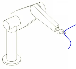
Figure 1. schematic diagram of the manipulator
The minimum time problem of tracking specified path by a serial manipulator was extensively studied by many researchers. Bobrow et al. [1] proposed a
method for time optimal motion of serial manipulators based on phase plane analysis. Considering that the solution is bang-bang in terms of acceleration along the path, the method reduces the problem into calculating the maximum and minimum acceleration along the trajectory in each step, and to find the switching points. They used a geometric approach in the phase plane and suggested a shooting method for finding switching points, in which one has to find a solution trajectory which comes in contact with the boundary of non-feasible region (NFR) without crossing it, where NFR is part of phase plane in which no solution that keeps end effector on prescribed trajectory is feasible. This procedure is numerically very difficult and expensive task to do.
changes signs. This advancement considerably reduced the numerical effort.
Zlajpah [3] introduced the concept of trapped area from which no solution trajectory can escape without leaving the prescribed trajectory, and locked area to which no solution trajectory can enter from within feasible area. Timar et al. [4] applied such methods to determine time-optimal solution for a CNC machine subject to prescribe acceleration bounds along axis. Sadigh and Hassan Ghasemi [5] showed that the lower boundary of these trapped and locked areas constructs the switching curve. The switching curve is a solution trajectory it-self, and could be generated by direct integration of equations of motion, provided that either the first switch or one of the critical points on it is known. The problem of minimum time motion along specified path for cooperative manipulators was also studied by several researchers. McCarthy and Bobrow [6] proved that for a manipulator with n coordinate, p differential constraint equations and m actuators, at least m-n+p+1
actuators are saturated during a time optimal movement along a prescribed path. Taking advantage of this result, Sadigh and Hasan Ghasemi [5] proposed a direct method for calculation of maximum and minimum acceleration for CMMS. Moon and Ahmad [7] em-ployed a similar algorithm as Bobrow et al. to find the time-optimal trajectory for a cooperative robot. They showed that to find the maximum and minimum values of acceleration at each point, one should solve a linear programming problem. They, however, did not elabo-rate on calculation of switching points, which itself is a very difficult part of the solution. Hasan Ghasemi and Sadigh [8] extended the work by Pfeiffer and Johanni to propose a direct method for computation of critical points for parallel manipulators and presented an algo-rithm to construct the switching curve. These advance-ments have made the situation for parallel manipulators similar to serial ones.
Minimum time motion of redundant manipulators along specified path is another interesting subject which has been studied in past two decades. Ma and Watanabe [9] and Galicki [10] extended the method proposed by Bobrow et.al. for serial redundant manipulators. They applied different secondary constraints such as heat characteristics and kinematic constraints to solve the problem.
Mattmüller and Gisler [11] presented a near time-optimal and jerk-constrained trajectory planner so that the constraint on the jerk translates into limits for the curvature of the phase-space velocity. Constantinescu and Croft [12] extended the time-optimal method to solve this problem with jerks constraints (limits on the rate of actuator torques) using perturbation trajectory improvement algorithm. Bianco and Piazzi [13] pre-sented a global optimization approach to obtain a minimum-time cubic spline trajectory for manipulator point-to-multipoint operations subject to constraints given by limited joint torques and torque derivatives. Osumi et al. [14] developed a time-optimal control method for quadruped walking robots and installed into a practical robot system. Yi et al. [14] presented a
pro-gramming method for time-optimal control of a mobile robot.
In spite of all above mentioned advancements in this area during last two decades, which made it possible to compute the maximum and minimum acceleration on line, switching points needs off line computation. This fact, which is due to computation of critical points, and backward integration for first and last switching points, prevents this method to be used as a control algorithm. So far the method can only be used for time optimal path planning.
This paper takes advantage of the previous theoretical developments in this area and presents a learning algo-rithm to find switching points and near-minimum time solution. The method can be used both for serial and parallel manipulators. Considering the fact that mini-mum time solution is bang-bang in terms of tangential acceleration, the basic idea behind the proposed method is to move the manipulator on the specified path on consequent segments of maximum acceleration, con-stant velocity, and maximum deceleration and to learn the manipulator to reduce and adjust the constant veloc-ity period in each step of learning process. As the con-stant velocity period gets smaller and smaller, the solu-tion converges the time optimal and two switches on the start and final time of constant velocity period con-verge the real switch. Adjustment of second switch also pushes the final error to zero. In fact, this method does not propose a new optimization algorithm, but it is a method to reduce calculation effort and backward inte-grations, necessary for finding switching points during a minimum time motion. This method substitutes the tedious numerical procedure of calculation of switching points with a simple learning process. As a result of this reduction in numerical effort, the method could be used online in practical problems. After this introduction, a brief statement of time-optimal problem along with phase-plane solution given by Dubowskey [1] is pre-sented in section two. The main idea of algorithm for single switch cases is discussed in third section. The fourth section is devoted to multi-switch cases followed by some numerical examples in fifth section.
2. Time Optimal Problem
Consider a non-redundant serial manipulator, which is supposed to move a payload from an initial point to a final point on a specified task space trajectory in mini-mum time subject to actuator's saturation limit. Motion of the payload in task space is defined by n coordinates;
]
,...,
[
X
1X
n
X
and the motion of the system isdefined with n variables; i.e.
q
[
q
1,...,
q
n]
T.The equations of motion of such system can be written as
1 1
1 ( , ) ( )
)
(
n n n n m m
n q q h qq B q τ
M (1)
In this equation, M, h, and τ are, respectively, the generalized mass matrix, coriolis and centrifugal terms, and the array of actuator forces.
q q J q q J X q q J X q p X ) ( ) ( ) ( ) ( (2)
Where q, p and J, respectively denote the array of joint coordinates, direct kinematic relation of the ma-nipulator and its Jacobian. On the other hand, the path can be expressed in terms of the non dimensional arc length variable, s, as
2 ) ( ) ( ) ( ) ( s s s s s s s f f X f X f X (3)
In above equations, f shows the relation of the path in task space with non dimensional arc length parameter,
s, also, (.)' denotes derivative with respect to s. Substi-tuting forX , X and X from equations (3) into equa-tions (2) and solving for q, q and q one gets:
)) ( ( 1f s
p
q (4)
s
s
J 1X J 1f( )
q (5)
s s s
s s
s
J 1X J 1JJ 1X J 1(f() f()2) J 1JJ 1f()
q (6)
Where P1 represent the inverse kinematics. Substitut-ing equations (4), (5) and (6) into equation (2), one can rewrite equations of motion as:
1 1 2 1 1 ~
n n n m m
n s d s e B τ
c (7)
The above system of equations represent n equations with two states,
s,s a similar formulation for a non-redundant parallel manipulator will result in equations of motion similar to equation (7); detailed formulation for such systems can be found in [8]. Any motion of the system, which moves the object on the prescribed path, must satisfy all above equations. Now, the optimization problem can be stated as:Problem (1): Find the desired path, s*(t), which
mini-mizes
f0
t
t dt subject to
m i s s s s s s i i
i 1,...,
) ( ~ ) ( ) ( ) ( max , min , 2 τ B e d
c
(8)
It can be shown, see Bobrow et al. [1], that the solution to this problem is bang-bang in s. To solve problem (1), one has to take the following steps:
1- Find the minimum and maximum acceleration at each step
2- Find the switching points and switch the acceleration at switching points.
It can be shown that all switching points are located on a switching curve [8], which for a specified manipulator is only a function of the desired trajectory. As stated in previous section there is no method for online calcula-tion of switching points. In next seccalcula-tion, we describe the proposed learning algorithm to find the switching points.
3. Single Switch Algorithm
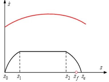
We assume that the described path is such that mini-mum time motion can take place with a single switch. As explained in first section, in the first step of learning algorithm we start the motion from
s
0 with maximum acceleration. The acceleration is then switched to zero at s1, see Figure 2, and motion is continued withcon-stant velocity until the end effector reaches point s2 along the path. At this point acceleration is switched to its minimum possible value and the motion is continued until the line
s
0
is crossed. With this planned mo-tion, one might expect s at final point to be different from desired one,s
f.Figure 2. schematic diagram of first step in learning process
Considering that the minimum time solution is bang-bang in terms of s, we know that the final solution is obtained if s2 coincide with s1. In other words, the solution is obtained once constant velocity portion of motion is totally eliminated and the manipulator is either moving with maximum acceleration or decelera-tion along the path. With this in mind, we must suggest a learning algorithm which can decrease the distance
between
s
1 and is
2 and to decrease the final error, if i e i
s
s
. The first action causes two approximate switching points s1 and s2 to converge to the exact switch and second action causes the end effector to stop at the desired final point. To make the algorithm clear we first propose separate algorithms for these two ac-tions and then try to combine them and present the final algorithm.3.1Elimination of Final Error
To eliminate the final error, assuming that minimum acceleration trajectories are almost parallel we may change the switching point si2 to s2ii at step i+1 which means
i i i
s
s 2
1
This correction continues until the final error becomes smaller than a reasonable value,
. Figure 3 shows thealgorithm of eliminating final error while
s
1 is kept i constant.Figure 3.schematic diagram of the process eliminating final errors
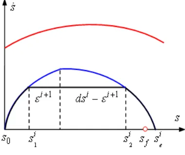
3.2Finding the Switching Point
To find the switching point, we increase s1, and de-crease s2 at each step until these, two converge to the single switch. To this end, at each step we change the switching points by a value of as follow
1 2 1 2
1 1 1 1
i i i
i i i
s s
s s
(10)
The value of i1 can be considered as follow ) ( 2 )
( 0 2 1 0
1
s s s s if s
s f
i i f
i
(11)
In which, is a constant which indicates how fast the switch points should approach each other in the early stages of the learning process, where the distance be-tween s1 and s2 is still larger than twice of . The value of should always be smaller than 0.5 and a good typical value for that would be some thing be-tween 0.05 to 0.2. Smaller values of means slower and safer approach to switch, while larger values of means faster approach to the switch but at the risk of crossing non-feasible region boundary; i.e. leaving the desired trajectory. Figure 4.a shows schematic graph of this algorithm.
As the learning process advances and two switches approach each other, their distance become smaller than
2 and it would not be possible to take the next step. In this case, considering the unsymmetric shape of the solution trajectory, see figure 4.b, we may assume that the distance of exact switch from s1i and si2 is different and is proportional to their distances travelled by maximum acceleration and maximum deceleration; i.e.,
i
s1 and sies2i. With this assumption one might
calcu-late i1 as:
) ( 2 )
(
2 2 1 0
1
1 if s s s s
ds s
ds s
f i i i
i e
i i
i
(12)
In which is a constant which shows how fast the switch points should approach each other at final stages of the learning process. The maximum value for is one and a good typical value for would be something between 0.75 to 0.9.
Figure 4.a. schematic diagram for algorithm of finding switching
Figure 4.b.schematic diagram for new value of i1
3.3Final Algorithm
At this stage, we may combine the above mentioned algorithms to obtain one which both approaches the approximate switches to the real one and to eliminate the final error. To this end, it is sufficient to make
cor-rections to
s
i2 based on both algorithms which meansi i i i
s
s21 2 1 (13)
Where
i and i are as defined in equation (9) to (12). Figure 5 shows how the final combined algorithm works.Figure 5.schematic diagram of results of minimum time algorithm
4 Multi Switch Algorithm
In this section, we consider the case where solution trajectory in phase plane enters non-feasible region; i.e. end effector leaves the prescribed path. For instance, suppose that at i1st iteration, solution trajectory en-ters NFR, as shown in Figure 6. In this case, in next learning iteration we simply try to perform the single switch algorithm once between points (s1i, si) and (sc1, si), and then between points (sc1, si) and (si2,
i
s ), see Figure 6. If in the process of finding these switches, the solution trajectory again intersects the NFR, a second critical point sc2 is introduced and similar algorithm of single switch is applied for that. To ensure escaping from crossing the NFR again and again it is suggested that i1 be reduced effectively. This means that in neighbourhood of a difficult portion of the path increase of velocity must be slowly.
5 Numerical Example
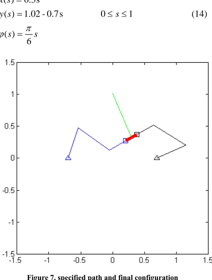
Figure 7 shows the schematic of a system composed of two planar manipulators handling a payload. The physical characteristics of the system are indicated in Table 1. Each manipulator has three DOFS. It is assumed that the payload is rigidly grasped such that no slipping or rotation is possible at contact points.
Figure 6.schematic diagram of multi switch algorithm
Table 1. physical characteristic of the system
5.1 Single Switch Problem
The system is assumed to move the payload on a pre-scribed path defined by equation (14), see Figure 7.
s s
s s
y s x
6 ) (
1 0 s
0.7 -02 . 1 ) (
s 0.3 ) (
(14)
Figure 7. specified path and final configuration
Exact solution obtained by forward integration with maximum acceleration from initial point and backward integration from final point results in 0.4693 as
m L m L L m L L m L
L1 40.5 , 2 50.6 , 3 60.3 , o0.2 kg m kg m m kg m m kg m
m1 41 2 51 3 60.3 o1
m N
T .
] 20 , 50 , 70 , 20 , 50 , 70 [ max
τ , τminτmax
switching point and 0.1647 as the total time elapse. This problem is solved taking advantage of the proposed method. The constant is considered to be
0.1 which means s11 is taken as 0.1 and 1 2
s
as 0.9. As one can see after four steps the conditions of) (
2 0
1
2 s s s
si i f is violated and i is reduced
from 0.1 to 0.047, and in next step to 0.0152. As the results in Table 2 show, approximate switches converge to the real switch after six steps of learning process. As can be seen this algorithm could obtain the switching time and the minimum time solution with no backward integration or length calculations. Figure 8 shows the final trajectory and boundary of non-feasible region for desired trajectory in phase plane.
Table 2.simulation results for single switch problem
Figure 8. simulation results of learning process in phase
plane
5.2Multi Switch Problem
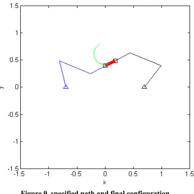
The system is assumed to move the payload on a circu-lar path defined by equation (15), see Figure 9.
s s
s s
s y
s s
x
5 . 0 ) (
1 0 62 . 0 ) 3 2 sin( 2 . 0 ) (
) 3 2 cos( 2 . 0 ) (
(15)
Figure 9.specified path and final configuration
Solution of this problem also starts based on the single switch algorithm stated in section 3 with 0.08. As one can see from Table 3, after two steps, the solution trajectory intersected the boundary of non-feasible region. As suggested in section4, we tried to find one switch before sc1 and one switch aftersc1. Simulation results for this process are given in Table 4. As one can see after 30 steps of learning process both switches on left and right of sc1 are converged. However, learning process for finding these switches are very costly. An-other point which worth mentioning is that the results obtained in first learning step is 10% more than the time elapse obtained from exact optimal solution of the problem, which is equal to 0.1981 sec. the next 30 steps of learning has reduced this 10% error to 1.3%. Figure 10 shows the final trajectory in phase plane as well as the non-feasible region boundary.
Exact solution to this problem by the conventional technique introduced by Bobrow et.al. [1] amounts to calculation of NFR boundary which needs a point to point calculation for each value of s from zero to one. Then the critical points on this boundary are to be cal-culated based on the algorithm introduced by Pfeiffer and Johanni [2] and Ghasemi and Sadigh [8]. Then one needs to perform direct integration from initial point and from critical points with maximum acceleration and backward integration from final point and critical points with maximum deceleration. The final step in the solu-tion would be to intersect generated trajectories to ob-tain exact switches. Comparing the simple calculations needed for comparing switching points in proposed algorithm with the lengthy and time consuming compu-tations necessary for obtaining exact switching points reveals the significance of proposed technique.
Table 3. numerical results for circular path before crossing BNF
step si
1
i
s2 dsisi2s1i
i
s i i contact ti
1 0.1000 0.9000 0.8000 5.6762 0.0800 0.0122 1 0.2182
2 0.1800 0.8032 0.6232 7.8189 0.0800 0.0122 0
Step si 1
i
s2 i i i s s
ds21 si i
iti
1 0.1000 0.9000 0.8000 6.3781 0.1000 0.0856 0.2188
2 0.2000 0.6815 0.4815 8.8294 0.1000 ‐0.0357 0.1698
3 0.3000 0.6239 0.3239 10.4794 0.1000 0.0168 0.1700
4 0.4000 0.5052 0.1052 11.6739 0.1000 ‐0.0209 0.1628
5 0.4470 0.4798 0.0328 12.0865 0.0470 ‐0.0117 0.1637
Figure 10. boundary of non-feasible region and solution path in phase plane
Table 4. numerical result of near minimum time motion
i
t
i b i b i b i
b s ds s
s1 2
i i a i a i a i
a s ds s
s1 2
step
0.2278
0.2019
0.196
0.2013
0.2011
0.2009
0.2007 0.5406 0.9900 0.4494 5.7351
0.7406 0.8028 0.0622 6.6891
0.7656 0.7977 0.0321 6.9572
0.7856 0.7860 0.0004 7.0930
0.7856 0.7860 0.0004 7.0930
0.7856 0.7860 0.0004 7.0930
0.7856 0.7860 0.0004 7.0930 0.1058 0.3998 0.2940 5.8781 0.0050
0.1168 0.3763 0.2595 6.1843 0.0050
0.1328 0.4107 0.2779 6.6381 0.0050
0.1398 0.1767 0.0369 6.8417 0.0050
0.1403 0.1792 0.0389 6.8515 0.0050
0.1408 0.1817 0.0409 6.9005 0.0050
0.1413 0.1842 0.0429 6.9005 0.0050
1
5
10
15
20
25
30
6. Conclusion
Problem of on line computation of switching points for a time optimal problem of a manipulator moving along a specified path is considered. The procedure can be used for on line evaluation of open loop time optimal control for both serial and parallel manipulators moving on a prescribed path. The method is based on the idea of moving end effector on the specified path on conse-quent segments of maximum acceleration, constant velocity, and maximum deceleration, and to learn the control to reduce and adjust the constant speed interval at each step of the learning process. This way two switches finally converge to the exact one and the final error is also eliminated. A development of the algo-rithm is also given for multi switch cases. The validity of the method is checked by solving time optimal prob-lem for two cases of a double three link planar parallel manipulator, along a straight line and then along a cir-cular line. The results for straight line show that in six steps of training, the final error is less than 0.44% and the travelling time is 0.28% more than the exact mini-mum time. These results are very promising both in accurate tracking and in fast learning process. Similar results are also reported for the circular path.
References
[1] Bobrow, J. E., Dubowsky, S. and Gibson, J.S.: Time-optimal control of robotic manipulators along specified
paths, Int. J. Robotics Res., 1985, vol.4, no.3, pp.3-17.
[2] Pfeiffer, F. and Johanni, R.: A Concept for Manipulator
Trajectory Planning, IEEE Journal of Robotics and
Automation, vol.RA-3, 1987, no.2, pp.115-123.
[3] Zlajpah, L.: On Time Optimal Path Control of
Manipula-tors with Bounded Joint Velocities and Torques, In Proc
of IEEE Int. Conf. on Robotics and Automation, Minnea-polis, 1996, pp.1572 - 1577.
[4] S. D. Timar, R.T. Farouki, and T.S. Smith, C.L. Boyad-jieff, Algorithms for time-optimal control of CNC ma-chines along curved tool paths, Robotics and
Computer-Integrated Manufacturing, 2005, 21, 37–53.
[5] Sadigh, M. J. and Ghasemi, M.H.: A Fast Algo rithm for Time Optimal Control of a Cooperative Multi
Manipula-tor System on Specified Path, in proc of 5th Vienna
sym-posium on mathematical modeling, modeling for/and con-trol, 2006, vol.2, pp.1-7.
[6] McCarthy, J. M. and Bobrow, J. E.: The Number of satu-rated Actuators and Constraint Forces During
Time-Optimal Movement of a General Robotic System, IEEE
Transaction on Robotics and Automation, 1992, vol.8, no.3, pp.407-409, June.
[7] Moon, S. B. and Ahmad, S.: Time-Optimal Trajectories for
Cooperative Multi-Manipulator System, IEEE
Transac-tion on system, Man and cybernetics, 1997, vol.27, no.2, pp.343-353.
[8] Ghasemi, M. H. and Sadigh, M. J.: A Direct Algorithm to Compute Switching Curve for Time Optimal Motion of Cooperative Multi-Manipulators Moving on Specified Path, International Journal of Advanced Robotics, 2008, vol.22, no.5, pp.493-506.
[9] S. Ma and M. Watanabe, Time-optimal control of kine-matically redundant manipulators with limit heat charac teristics of actuators, Advanced Robotics, 2002, vol.16, no.8, pp.735 – 749
[10] M. Galicki, Control of kinematically redundant manipu-lator with actuator constraints, Robot Motion and Con-trol,in proc of the Fifth International Workshop (RoMoCo '05), 2005, pp.123- 130.
[11] J. Mattmüller and D. Gisler, Calculating a near time-optimal jerk-constrained trajectory along a specified smooth path, International Journal of Advanced
Manu-facturing Technology, 2009, 45, 1007–1016.
[12] D. Constantinescu and E. A. Croft, Smooth and time op-timal trajectory planning for industrial manipulators along specified paths, Journal of Robotic Systems, 2000, 17, 233-249.
[13] Bianco, C. G. L. and Piazzi, A. Minimum-time trajectory planning of mechanical manipulators under dynamic con-straints, International Journal of Control, 2002, 75(13), 967-980.
[14] H. Osumi, S.Kamiya, H. Kato, K. Umeda, R. Ueda, and T. Arai, Time optimal control for quadruped walking ro-bots, in Proc. IEEE International Conference on Robotics
and Automation, 2006, Orlando, pp. 1050-4729.
[15] F. Y. Yi, K. CH. Nan, L. T. Li, and W. CH. Ju, A Nonlin-ear Programming Method for Time-Optimal Control of an Omni-Directional Mobile Robot. Journal of Vibration
Biography of Authors
Mohammad Jafar Sadigh received his B.S. and M.S. degrees in Me-chanical engineering both from Isfahan University of Technology (IUT), Isfahan, Iran in 1986 and 1989, respectively, and PhD from McGill University Montreal, Canada in 1995. Since 1995 he has been with the Department of Mechanical engineering at Isfahan University (IUT), Isfahan, Iran. His research interests are system dynamics, control of dynamical systems, robotics, and also he is very active in the field of science park development and technology manage-ment.
(Email: [email protected])