University of New Orleans University of New Orleans
ScholarWorks@UNO
ScholarWorks@UNO
University of New Orleans Theses and
Dissertations Dissertations and Theses
8-8-2007
Frequency Estimation Using Time-Frequency Based Methods
Frequency Estimation Using Time-Frequency Based Methods
Cuong Mai
University of New Orleans
Follow this and additional works at: https://scholarworks.uno.edu/td
Recommended Citation Recommended Citation
Mai, Cuong, "Frequency Estimation Using Time-Frequency Based Methods" (2007). University of New Orleans Theses and Dissertations. 571.
https://scholarworks.uno.edu/td/571
Frequency Estimation Using Time-Frequency Based
Methods
A Thesis
Submitted to the Graduate Faculty of the University of New Orleans in partial fulfillment of the requirements for the degree of
Master of Science in
Engineering Electrical Engineering
by
Cuong Mai
B.S. University of New Orleans, 2003
TABLE OF CONTENTS
LIST OF FIGURES... iii
ABSTRACT...v
INTRODUCTION... 2
CHAPTER 1... 3
CURRENT METHODS FOR ANALYZING INSTANTANEOUS FREQUENCY... 3
CHAPTER 2... 28
PROPOSED METHOD ... 28
CHAPTER 3... 32
RESULTS AND ANALYSIS... 32
CHAPTER 4... 65
REAL-TIME HARDWARE IMPLEMENTATION ... 65
CHAPTER 5... 77
CONCLUSIONS... 77
BIBLIOGRAPHY... 79
APPENDIX A... 80
APPENDIX B... 83
APPENDIX C... 87
LIST OF FIGURES
Figure 1 : 3-D parameter space based on the use of multiple windows... 4
Figure 2: Chirp and Chirplet in time (Real and Imaginary components) (Image by Mann and Haykin) [6]... 7
Figure 3: Time-Frequency scale of Chirp and Chirplet (Image by Mann and Haykin) [6] ... 8
Figure 4: 3-dimensional helix view of Chirp and Chirplet in time... 8
Figure 5: An original chirp function (Image by Angrisani and D’Arco) [7] ... 9
Figure 6: Chirping in Time (Image by Angrisani and D’Arco) [7]... 10
Figure 7: Chirping in Frequency (Image by Angrisani and D’Arco) [7] ... 11
Figure 8: Time translation g(t – tc) (Image by Angrisani and D’Arco) [7] ... 11
Figure 9: Frequency Translation (Image by Angrisani and D’Arco) [7] ... 12
Figure 10: Frequency dilation/ time contraction represented by 1 1 | t| t g ∆ ∆ (Image by Angrisani and D’Arco) [7] 12 Figure 11: a) Time-Frequency plot from a traditional Chirplet Transform. b) Time-Frequency plot from a modified Chirplet Transform (Image by Angrisani and D’Arco) [7] ... 16
Figure 12: Test signal s(t) in the time domain (Plot by Angrisani and D’Arco) [7]... 19
Figure 13: Time-frequency plot of result obtained from the traditional Chirplet Transform (Plot by Angrisani and D’Arco) [7]... 19
Figure 14: Time-frequency plot of result obtained from the modified Chirplet Transform (Plot by Angrisani and D’Arco) [7]... 20
Figure 15: Time plot of two component test signal (Plot by Angrisani and D’Arco) [7] ... 20
Figure 16: Result obtained from Modified Chirplet Transform on a two component signal (Plot by Angrisani and D’Arco) [7]... 21
Figure 17: Result obtained from reassigned STFT on a two component test signal (Plot by Angrisani and D’Arco) [7] ... 21
Figure 18: Test signal s(t) of a bat sound used for approximation (Image by Qian and Chen) [9]... 26
Figure 19: Spectrogram of results obtained with Chirplet Based Adaptive Approximation (5 chirplets) (Image by Qian and Chen) [9] ... 27
Figure 20: Test signal with linear chirp rate = 0.001 start at 200 Hz, Sampling Frequency = 8000 ... 35
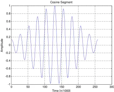
Figure 21: Example of Gaussian Windowed Cosine Segment Used for Projection ... 36
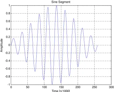
Figure 22: Example of Gaussian Windowed Sine Segment Used for Projection... 37
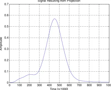
Figure 23: Example of Signal Resulting from Projection Used for Peak Detection. (The highest peak indicates matching frequency found. Other low peaks will be discarded by applying a threshold) ... 38
Figure 24: Results from Proposed Method with Peak Detection (Window Size = 10*Period of i, τ = 1 Scanning Frequency Range i = 100-4000Hz with Interval of 10Hz)... 39
Figure 25: Results from Proposed Method with Peak Detection (Window Size = 4*Period of i, τ = 10 Scanning Frequency Range i = 100-4000Hz with Interval of 5Hz)... 40
Figure 26: Results from STFT (Spectrogram) by MATLAB (Window Size = 64, FFT size = 1024, 50% overlapped)... 41
Figure 27: Test signal with quadratic chirp rate = 0.00001 start at 300 Hz, Sampling Frequency = 8000 ... 42
Figure 28: Results from Proposed Method with Peak Detection (Window Size = 2*Period of i, τ = 1, Scanning Frequency Range i = 100-4000Hz with Interval of 100Hz)... 43
Figure 29: Results from Proposed Method with Peak Detection (Window Size = 4*Period of i, τ = 10, Scanning Frequency Range i = 100-4000Hz with Interval of 5 Hz ... 44
Figure 31: Results from STFT (Spectrogram) by MATLAB (Window Size = 32, FFT size = 1024, Overlapped Size =
30) ... 46
Figure 32: Test signal with quadratic chirp rate = 0.00002 start at 300 Hz, Sampling Frequency = 16000 Hz... 47
Figure 33: Results from Proposed Method with Peak Detection (Window Size = 4*Period of i, τ = 1, Scanning Frequency Range i = 100-4000Hz with Interval of 100 Hz, Cosine Projection Only) ... 48
Figure 34: Results from Proposed Method with Peak Detection (Window Size = 4*Period of i, τ = 10, Scanning Frequency Range i = 100-4000Hz with Interval of 10 Hz, Cosine Projection Only) ... 49
Figure 35: Results from Proposed Method with Peak Detection (Window Size = 4*Period of i, τ = 10, Scanning Frequency Range i = 100-4000Hz with Interval of 10 Hz, Cosine and Sine Projection) ... 50
Figure 36: Results from Proposed Method with Peak Detection (Window Size = 2*Period of i, τ = 10, Scanning Frequency Range i = 100-4000Hz with Interval of 10 Hz, Cosine and Sine Projection) ... 51
Figure 37: Results from STFT (Spectrogram) by MATLAB (Window Size = 100, FFT size = 1024, Overlapped Size = 50) ... 52
Figure 38: Test signal with linear chirp rate = 0.001 start at 1000 Hz, Sampling Frequency = 8000 Hz... 53
Figure 39: Results from Proposed Method With Peak Detection (Window Size = 6*Period of i, τ = 1, Scanning Frequency Range i = 100-4000Hz with Interval of 10 Hz, Cosine and Sine Projection) ... 54
Figure 40: Results from STFT (Spectrogram) by MATLAB (Window Size = 64, FFT size = 1024, Overlapped Size = 32) ... 55
Figure 41: Test signal with linear chirp = 0.001 start at 1000 Hz and 1300 Hz, Sampling Frequency = 8000 Hz... 56
Figure 42: Results from Proposed Method with Peak Detection(Window Size = 8*Period of i, τ = 1, Scanning Frequency Range i = 100-4000Hz with Interval of 10 Hz, Cosine and Sine Projection) ... 57
Figure 43: Results from STFT (Spectrogram) by MATLAB (Window Size = 64, FFT size = 1024, Overlapped Size = 32) ... 58
Figure 44: Test signal with linear chirp = 0.002 and quadratic chirp = 0.00003 start at 1000 Hz and 500 Hz, respectively. Sampling Frequency = 16000 Hz... 60
Figure 45: Results from Proposed Method with Peak Detection (Window Size = 8*Period of i, τ = 1, Scanning Frequency Range i = 100-8000Hz with Interval of 10 Hz, Cosine-Sine Projection)... 61
Figure 46: Results from STFT (Spectrogram) by MATLAB (Window Size = 16, FFT Size = 1024, 100% Overlapping) ... 62
Figure 47: Results from STFT (Spectrogram) by MATLAB (Window Size = 128, FFT size = 1024, 100 % Overlapping) ... 63
Figure 48: Results from Proposed Method before Peak Detection (Window Size = 8*Period of i, τ = 1, Scanning Frequency Range i = 100-8000Hz with Interval of 10 Hz, Cosine-Sine Projection)... 64
Figure 49: TMS320C6713 DSP Development Board (Image by Texas Instruments, Inc.) ... 66
Figure 50: Code Composer Studio Interface... 68
Figure 51: Setting the Number of Samples per Buffer Size... 69
Figure 52: Configure Setting for Software Interrupt Intervals... 72
Figure 53: Input Signal for Hardware Testing (Frequency = 1000 Hz, Sampling Rate = 8000 Hz, Chirp-rate = 0.001) ... 74
Figure 54: Output Signal by Hardware Testing (128 Samples/Buffer, τ = 9, i = 200 to 2000 Hz with 100 Hz Interval, Cosine Only) ... 74
Figure 55: Input Signal for Hardware Testing (Frequency = 1000 Hz, Sampling Rate = 8000 Hz, Chirp-rate = 0.002) ... 75
ABSTRACT
Any periodic signal can be decomposed into a sum of oscillating functions. Traditionally, cosine
and sine segments have been used to represent a single period of the periodic signal (Fourier
Series). In more general cases, each of these functions can be represented by a set of spectral
parameters such as its amplitude, frequency, phase, and the variability of its instantaneous spectral
components. The accuracy of these parameters depends on several processing variables such as
resolution, noise level, and bias of the algorithm used. This thesis presents some background of
existing frequency estimation techniques and proposes a new technique for estimating the
instantaneous frequency of signals using short sinusoid-like basis functions. Furthermore, it also
shows that the proposed algorithm can be implemented in a popular embedded
DSP-microprocessor for practical use. This algorithm can also be implemented using more complex
features on more resourceful processing processors in order to improve estimation accuracy.
Keywords: frequency estimation, oscillating functions, Digital Signal Processing, instantaneous
INTRODUCTION
Instantaneous frequency estimation is a signal processing component which is vital for many
application fields, including analysis of radar signals, seismic reflection, and electromagnetic
interference [1]-[4]. Instantaneous frequency is defined as the derivative of the argument f(t) of a
signal having the form cos(f(t)), namely df t( )
dt . Precise interpretation of complex signals that
consist of various time-frequency structures requires decomposing the signals into parametric,
redundant, and well-localized components in the time-frequency plane. These localized functions
are often called time-frequency atoms. Decomposing signals in time-frequency components gives
important information about the signal, when such information cannot be obtained by using the
classical time-domain or frequency-domain analysis methods [5]. For instance, rotation and
shearing [7] characteristics of frequency-varying signals can be obtained in the time-frequency
plane, as it will be discussed in detail in Chapter 1.
This thesis presents an overview of instantaneous frequency estimation methods, including those
based on Short Time Fourier Transform (STFT), Wavelet Transform, and Chirplet Transform.
Then, two practical methods of Chirplet Transform-based frequency estimation for
multi-component signals are discussed. A new method is proposed, and its hardware implementation on
a TI6713 board is discussed. The limitations and strengths of the hardware used are also discussed.
Moreover, a MATLAB implementation is presented with the purpose of expanding the proposed
CHAPTER 1
CURRENT METHODS FOR ANALYZING
INSTANTANEOUS FREQUENCY
I. Short Time Fourier Transform (STFT) and Wavelet Transform
In the recent past, researchers became aware of the limitations of frequency-domain methods. The
Fourier Transform (FT), which was traditionally used for frequency analysis, was able to yield
perfect reconstruction of signals; however, it was not able to provide a meaningful interpretation of
the signal’s frequency content in the case where the signal varies with time. Later, researchers
focused on time-localized methods which allowed them to observe how the signal’s spectrum
evolves over time by performing frequency analysis within short time signal segments. These
methods are called time-frequency (TF) methods. One of these methods is the short-time Fourier
transform (STFT). This method involves computing the FT of a signal s(t) using a window of short
duration. The process is repeated for different shifts of the window, thus obtaining the spectrum of
the signal at different time intervals. A multiple-scale version of this approach involved stretching
Figure 1, stacking these STFT’s on top of one another results in a continuous volumetric
representation of the signal s(t), which is a function of time, frequency, and window size [6].
Figure 1 : 3-D parameter space based on the use of multiple windows
Another time-frequency representation is the Wavelet Transform which involves computing the
inner product of the signal s(t) under analysis with a family of translates and dilates of one basic
primitive called the mother wavelet. A member of the wavelet family is produced by a particular
1-D affine coordinate transformation acting on the time axis of the mother wavelet. This geometric
transformation is parameterized by two numbers corresponding to the amounts of translation and
dilation. By taking the inner products of the signal s(t) with many members of the two-parameter
wavelet family, the continuous wavelet transform is formed [6].
. . .
Time
F
re
q
u
en
II. Chirplet Transform
A different approach for obtaining a time-frequency representation of s(t) is based on the
decomposition of s(t) using basis functions. This approach is based on an assumption that, in
general, a signal can be expressed as a weighted sum of mono- component signals. In the case of
the FT representation, these mono-component signals are single frequency components represented
by Aej tω , where ω is the component’s frequency, and A is its amplitude. The Chirplet Transform
approach uses a different representation of the signal components, which in this case are called
chirplets. It will be discussed in detail in section II.1 that chirplets are short-timed signals that
depend on several parameters, in contrast to the single-frequency components, Aej tω , used in FT,
and to the wavelets used in Wavelet Transforms.
The concept of Wavelet Transform and Fourier Transform processing is similar to that of Chirplet
Transform processing, in the sense that the original signal is projected on a set of basis functions.
The Chirplet Transform, as formulated by Mann and Haykin [6] is “a multi-dimensional parameter
space whose coordinate axes correspond to the pure parameters of planar affine coordinate
transformations in the time-frequency plane.” Compared to other linear Time-Frequency
representations, such as STFT or the Wavelet Transform, the Chirplet Transform represents 1-D
time-domain signals by multi-dimensional functions. Most often, the function is five-dimensional,
• amplitude scaling,
• chirping in time,
• chirping in frequency,
• shearing in time,
• shearing in frequency.
The mapping of a signal in the five-dimensional space, whose dimensions are defined above, helps
to overcome the resolution problem from which other time-frequency representations suffer [7].
II. 1. Gaussian Chirplet
A simple chirplet can be derived by applying simple mathematical operations to a Gaussian
enveloped function. The function can be thought of as the primitive that generates a family of
chirplets. The primitive function is defined as follows:
2
(1/ 2)( / ) 2 ( ) , ,
1
( )
2
c c c c c
t t j f t t j t f
g
σt
e
σe
π φπσ
− − − +
′
=
(1)where j= −1,tc∈ℜ is the center of the energy concentration in time; fc∈» is the center
frequency, σ∈»>0 is the spread of the Gaussian envelope, and φ∈» is called the phase shift.
The three subscripts of function g’ represent the three chirplet’s degrees of freedom. If the
primitive function is required to have unit energy, it needs to be raised to ½ and multiplied by an
appropriate normalization constant. The phase parameter φ does not appear in (2) for the purpose
2
2 1
1
2
2 ( ) [ 2 ( )]
2 , , 1 1 ( ) 2 c c t
c c c c
c c
t t t t
j f t t j f t t
t f
t
g σ t e σ e π e e π
πσ π − − − − ∆ − − ′ = = ∆ (2)
where ∆ =t 2
σ
This primitive function can also be thought of as the product of an envelope and the harmonic
oscillation component. A family of Gaussian chirplets is formed by retaining the envelope of the
primitive and replacing the harmonic oscillation with a linear frequency modulated chirp. For
example:
2
2 1
2 2 [ ( ) ( )] , ,log( ),
1 ( )
c
t c c c
c c t
t t
j c t t f t t
t f c
t
g t e e π
π − − ∆ − + − ∆ = ∆ (3)
The expression above defines a Gaussian chirplet with four parameters: time center tc, frequency
center fc, log-duration log (∆t), and chirprate c [6].
A chirp and a chirplet in time are shown in Figure 2.
Figure 3: Time-Frequency scale of Chirp and Chirplet (Image by Mann and Haykin) [6]
CHIRP CHIRPLET
Figure 4: 3-dimensional helix view of Chirp and Chirplet in time
Figure 3 shows the chirp and chirplet in the time-frequency scale. The chirp is characterized by a
linear increase in frequency. Figure 4 shows a 3-D helix view of the chirp and chirplet as they
change in time. As shown in Figure 3 (right), a chirplet is represented as a cell of ellipsoidal shape.
The chirplet also has the same linear increase in frequency but with varying amplitude (growing
II.2. Chirplet Operators
The Chirplet Transform is capable of rotating each cell of the time-frequency plane similar to the
one shown in Figure 4, as well as shearing it along the time and frequency axes. The Chirplet
Transform’s capability of shaping the time-frequency cells presents new opportunities of
optimizing the time-frequency resolution according to the analyzed signal. For example, it is
possible to rotate and shear each cell according to the local slope of the trajectory of the analyzed
instantaneous frequency, thus giving the opportunity of better tracking the frequency’s evolution
versus time. These degrees of freedom are provided by modifying the chirp’s parameters in order
to perform basic chirp operations such as the ones described next:
a. Chirping in time
Chirping in time is obtained by multiplying the mother chirplet (Figure 5), or the primitive
function, g(t) with a linear Frequency Modulated (FM) signal, chirp (
2 2
2 c j t
e π ) where c is the
chirp-rate. It causes a rotation of each cell as well as its shear along the frequency axis. The rotation
angle with respect to the time axis is α which depends on the chirp-rate c. The slope of the cell on
the time-frequency plane is equal to the value of c (Figure 6) [7].
Figure 6: Chirping in Time (Image by Angrisani and D’Arco) [7]
b. Chirping in frequency (time shearing)
Chirping in frequency (time shearing) [6] is given by convolving, in the time domain, the mother
chirplet g(t) with another FM linear chirp
(
)
2 1 1 2
2 2
j t
d jd − e π
− where the parameter d accounts for the
shear amount along the time axis imposed on the cell. In the frequency domain, this is
accomplished by multiplying the Fourier Transform of the mother chirplet, G(t), and the function
2 2
2 d j f
e− π which can be considered a chirp in the frequency domain with the chirp-rate equal to d
[7]. The rotational angle with respect to the frequency axis is β which depends on the chirp-rate d.
Figure 7: Chirping in Frequency (Image by Angrisani and D’Arco) [7]
c. Time translation
Time translation is done by shifting the mother chirplet g(t) by tc in time where tc is the time offset
[7].
Figure 8: Time translation g(t – tc) (Image by Angrisani
and D’Arco) [7]
d. Frequency-translation:
Frequency translation is done by multiply the mother chirplet g(t) by ej2πfct or g(t)ej2πfct where fc is
Figure 9: Frequency Translation (Image by Angrisani and D’Arco) [7]
e. Dilation in Frequency/ Contraction in Time:
Changing the sampling rate or resolution of the signal in time cause the cell to be either dilated or
contracted in time. When that happens, the reverse effect is caused in the frequency scale [7].
Figure 10: Frequency dilation/ time contraction
represented by
1 1 | t| t
g
∆
∆ (Image by Angrisani and
D’Arco) [7]
All of the above operations can be combined to a complete analytic expression of the Chirplet
Transform of a signal s(t):
with the kernel h(τ) given by:
(5)
The full continuous chirplet transform (CCT) can also be written using a different notation as:
S
tc,fc,log(∆t), ,c d=
C
tc,fc,log(∆t), ,c dg t
( ) | ( )
s t
(6)where tc, fc, log(∆t), c, d are the time shift, frequency shift, resolution (based on window size),
chirp-rate in time, and chirp-rate in frequency.
For any operator in the time domain, there is an equivalent operator in the frequency domain or in
the time-frequency plane or in any other reasonable coordinate space in which one wants to work
in. When using more than one operator, it should be cautioned that operators do not commute,
including the frequency-shift and time-shift operators. For example, if time-shift is applied first and
then frequency shift is applied next. This is not equivalent to applying a frequency shift followed
by a time shift, since the result would contain a different phase shift [6].
2 2 ( ) 2 ( ) 1 ( , , , , )
t : time f: frequency
a: scaling parameter
c c c
t t v
j f t c v
a d
c c c
t t
h t t f a c d g v e dv
III. CHIRPLET TRANSFORM AND FREQUENCY ESTIMATION
The Chirplet Transform projects the input signal onto a set of functions that are obtained by
modifying an original function g(t), or the mother chirplet as described in Part II. The most popular
chirp operators being used are time shifting, frequency shifting, scaling, chirping in time, and
chirping in frequency [7]. Because of the variety of operators being used, the Chirplet Transform
reveals more information about the original signal s(t) compared to the traditional FT. However,
Chirplet Transform can be very time-consuming since each chirplet parameter’s range must be
large enough to obtain a large number of chirplets.
IV. MODIFIED CHIRPLET TRANSFORM FOR INSTANTANEOUS
FREQUENCY ESTIMATION
IV.1. Mathematical derivation
Angrisani, L. and D’Arco, M. proposed a method of modified Chirplet Transform to improve the
shape and aspect ratio of the time-frequency cell, to better match the local features of the analyzed
signal [7]. To accomplish this, a modification of the mother chirplet, g(t) is introduced by
multiplying the chirplet function by the following term:
3
2 6 k j t
e
π (7)where k is the curvature parameter.
enable the Chirplet Transform to track the evolution versus time of the instantaneous frequency of
each analyzed component more closely in the presence of instantaneous frequencies characterized
by high dynamics. The authors also claimed that in high dynamic environments, this modified
version of Chirplet Transform achieves better resolution than the linear approximation provided by
the traditional Chirplet Transform [7].
In particular, the authors proposed using a Gaussian window function as the mother chirplet to
achieve the best time-frequency resolution. Its expression is:
2
1 2
1 ( )
2
t
g t e σ πσ
−
= (8)
This mother chirplet has unit energy and the parameter σ accounts for its time extent. In Figure
11b, the noticeable bending of the time-frequency cell is visible. This bending effect is claimed by
the authors as effectively corresponding to the trajectory points of the analyzed signal (in the
time-frequency plane). Moreover, because the time-time-frequency cell representation of this mother chirplet
has elliptical contours on the time-frequency plane, analyzing chirping in frequency is not
necessary. On the other hand, the scaling parameter, a, at any point in the time-frequency plane has
to establish only the aspect ratio of the cell centered at that point, not the position of the cell along
Figure 11: a) Time-Frequency plot from a traditional Chirplet Transform. b) Time-Frequency plot from a modified Chirplet Transform (Image by Angrisani and D’Arco) [7]
The final expression of the kernel, h (t-tc, fc, a, c, d), of the modified Chirplet Transform is:
2 2 3 1 ( ) ( ) ( ) 2 3 1 ( , , , , ) 2 c
c c c c
t t k
j f t t c t t t t a
c c
h t t f a c k e e
a π σ
π σ
− − − + − + − − = × (9)
2. Computer Algorithm
a. Chirp-rate Establishment
Initially, a traditional Chirplet Transform with no chirping in time (c=0), no bending effect (k=0),
and unitary scale parameter (a = 1) is evaluated for each ∆t of the test signal. The results give a
rough estimate of how many components the signal consist of. A peak location algorithm [8] is
applied to the same results to obtain a coarse time evolution of the instantaneous frequency of each
component. Then, the slope at each point (t*, f*) on the time-frequency plane is evaluated. This
2 1 2 1 f f r
t t
− =
− (10)
where ( f t ) 2, 2 and ( , )f t1 1 are the coordinates of the two points of the same trajectory that are close
to (t*, f*) so that *
1 2
t <t <t and *
1 2
f < f < f .
The value of r characterizing a generic point (t*, f*) of each reconstructed trajectory is equal to the
value of the chirp rate c which characterizes the cell centered at the same point in the
time-frequency plane [7].
b. Curvature Evaluation
Subsequently, for each time-frequency point at (t*, f*), a Gaussian mother chirplet is established
with time and frequency shifted by t* and f*, respectively. Chirping in time is also applied with
chirp rate r. Then, the value of the curvature parameter, k, for the same cell is iteratively
incorporated into the mother chirplet using (12). Finally, the mother chirplet is projected onto the
signal until the results reach a maximum. The value of k which results in that maximum will be the
desired curvature value of the cell [7].
c. Scaling Adjustment
Lowering the value of the scale parameter, a, results in reducing the value of ∆t. The values of the
test signal. These properties are used for computing the scaling factor for the cell on the
time-frequency plane [7].
d. Instantaneous Frequency Estimation
Frequency estimation is done by using the values of the chirp rate, curvature, and scale obtained
previously to characterize all the points in the time-frequency plane belonging to the cell centered
at (t*, f*). The process is repeated for the remaining points of the time-frequency plane. To
efficiently accomplish this, the authors suggested generating a map of the optimal values of
parameters throughout the time-frequency plane. The modified Chirplet Transform of the signal is
evaluated by making use of the mapped parameter values to reconstruct the trajectory of each
component’s instantaneous frequency. An enhanced peak location algorithm is suggested by the
authors to perform this reconstruction [7].
3. Testing and Results
a. Test on Mono-component signals
Testing was conducted by the authors on a mono-component signal which has the following
expression in the time domain:
s(t) = a(t)x(t) where 0 < t < 102.4 µs ;
2 5 5*10 28
15
( )
t
a t
e
π −
−
=
6 10 2 15 3 19 4
( ) cos[2 (2.004 10 7.26 10 1.1882 10 5.375 10 )]
x t =
π
⋅ t− ⋅ t + ⋅ t − ⋅ tFigure 12: Test signal s(t) in the time domain (Plot by Angrisani and D’Arco) [7]
The results acquired in the time-frequency plane using the traditional and modified Chirplet
Transform are shown in Figure 13 and Figure 14, respectively. The noticeable bend can be
observed clearly in the result from the modified Chirplet Transform. The authors stated that the
maximum difference between the test signal and the synthesized signal from the modified Chirplet
Transform is about 1% while it is 3% for the traditional Chirplet Transform [7].
Figure 14: Time-frequency plot of result obtained from the modified Chirplet Transform (Plot by Angrisani and D’Arco) [7]
b. Test on multi-component signal
A test was conducted by the authors on a test signal which has two components [7] with the
following expression:
6 10 2 13 3
16 10 2 13 3
( ) ( ) ( ) 0 102.4
( ) cos[2 (1.9041 10 1.0252 10 3.482 10 )]
( ) cos[2 (2.0041 10 1.0252 10 3.482 10 )]
s t x t y t t s
x t t t t
y t t t t
µ
π
π
= + < <
= ⋅ − ⋅ + ⋅
= ⋅ − ⋅ + ⋅
The same sample rate (5 Msamples/s) and the same number of samples (512 samples) were used
for this test. Figure 15 shows the graphical plot of the input signal in time.
The result (Figure 16) is then compared with the result from a reassigned STFT on the same test
signal in Figure 17. Using these results to reconstruct the trajectories in both cases, the
reconstructed trajectories in the case of the modified Chirplet Transform are observed as smooth
and continuous for both components while they are observed as abrupt and partially visible when
using STFT. As a result, the authors concluded that the modified Chirplet Transform performed
better than STFT at separating multiple closely-spaced spectral component signals [7].
Figure 16: Result obtained from Modified Chirplet Transform on a two component signal (Plot by Angrisani and D’Arco) [7]
V. Adaptive Chirplet Based Signal Approximation
1. Adaptive Approximation
Another method of frequency estimation is proposed by Qian S. and Chen, D. using Adaptive
Chirplet combined with the Wigner-Ville distribution [9]. It begins with the assumption that the
test signal s(t) can be represented as:
1
1 0
( )
( )
( )
p
p p p
p
s t
A h t
s
t
−
+ =
=
∑
+
(11)where
1( ) ( ) ( )
p p p p
s + t =s t −A h t ; s0 =s t( ); Ap =
∫
s t h t dtp( ) p( ) . Apis the inner product of the signal s(t)and the chirplet hp(t); sp(t) is the residual after the orthogonal projection Ap has been removed from
the original signal s(t).
In addition, the chirplet hp(t) is chosen so that
2 2
1
min ( ) min ( ) ( )
p p
This approach guarantees that the residual sp+1( )t 2monotonically decreases as the number of
terms, p, increases. When p is large enough and the number of samples is finite, the residual may
reduce to zero [9]. In order to reduce the residual, the following equation needs to be solved:
2 2
max
max
( )
( )
p p
h
A
p=
h∫
s t h t dt
p p (13)However, solving the optimization problem in (13) is difficult. Therefore, hp(t) has to be limited to
be a frequency modulated Gaussian function (14) with βp = 0
2 2
1/ 4
( ) / 2 ( / 2)
( )
p p t tp j pt ptp
a
h t
e
α ω βπ
− − + +
=
(14)where α, tp, ωp, β are the scaling, time offset, frequency offset, and chirp rate, respectively.
Since the residue sp+1( )t 2converges as the number of terms increases, the authors claimed it can
be neglected when it is small enough in practical applications [10]. Therefore, (11) can be reduced
to:
0
( )
p p( )
p
s t
A h t
∞
=
=
∑
(15)The authors then suggested using the zooming algorithm to estimate the optimal chirplet. The
zooming algorithm involves the use of a Gaussian function to scan (to project the Gaussian
deviation and center parameters of the Gaussian function are adjusted until a smallest deviation can
be found with the highest peak. Finally, the outputs of the zooming algorithm are:
• The time variance 1/d, where d ≥αp.
• The center time tc = tp
• The center frequency ωc = ωp
The Wigner-Ville distribution is then applied to the Gaussian chirplet to obtain a time-frequency
representation. Its expression is:
2 2
( ) ( ) /
( , )
2
p t tp p pt pp
WVD t
ω
=
e
−α − −ω ω− −β α (16)where WVDp(t,ω) is the Wigner-Ville distribution of the signal s(t).
Equation (16) is then used to compute the power spectrum of hp(t). The power spectrum is
computed as:
2
2 ( ) /
( )
( , )
2
p p pt cp p
H
WVD t
dt
e
c
ω ω β
π
ω
=
∫
ω
=
− − − (17)In addition, the width of the power spectrum of hp(t) is proportional to the chirp rate |βp| (the width
increases as |βp| increases).
Furthermore, this power spectrum is a Gaussian function which has center frequency at
c p p pt
ω =ω +β (18) (estimated by the zooming algorithm). Its variance is formulated as
(19). As a result, when βp = 0, the variance is αp = d where 1/d is the time variance estimated by
the zooming algorithm [9].
2. Computer Algorithm
The authors suggested that the adaptive approximation algorithm can be implemented as follow:
a. Apply the zooming algorithm to estimate the time variance t/d, center time tc, and center
frequency ωc.
b. Compute the signal’s power spectrum using (17).
c. Estimate the frequency variance of the Gaussian function center at ωc.
d. If the variance equals to d, then βp =0, αp =d =variance, tc = tp, ωc =ωp. If not, go to step e.
e. Set the initial value of αp to d.
f. Compute βp (chirp rate) by (19) and ωc (center frequency) by (18).
g. Construct hp (t) with found parameters using (14).
h. Compute the inner product of hp(t) and sp(t) using (15).
i. Reduce αp by a small quantity of ∆α (αp = αp - ∆α) and repeat step f to step h until αp = 0. The
parameters (αp, tp, ωp, βp) corresponding to the largest |Ap|2 constitute the optimal chirplet
hp(t).
The negative outcome of this algorithm above is that it can be very computationally intensive
which may not be suitable for embedded processors with real-time processing. As described above,
step i is the most time consuming because of the iterative decrement of parameter αp and the
estimation accuracy depends on the amount of ∆α. However, because |Ap|2 is less sensitive to small
3. Testing and Results
Tests on this method were done by the authors on an echo-location pulse test signal emitted by a
large brown bat. The signal was digitized into 400 samples and its plot in the time domain is in
Figure 18. Subsequently, the relative residual used for approximation is defined
as
2
2
( )
100 ( )
p s t residual
s t
= × .
Figure 18: Test signal s(t) of a bat sound used for approximation (Image by Qian and Chen) [9]
As shown the image, the test signal is clearly a chirp signal with a nearly smooth Gaussian envelop
which is perfect for the purpose of testing this Adaptive Approximation method. The expected
result is also expected to be smooth with negative slope in the time-frequency plot. The authors
subsequently performed the tests on a Pentium 120 PC [9]. The test signal s(t) was approximated
and represented by five chirplets. The test then reportedly ran for 0.49 second producing final
residuals of less than ten percent. Those residuals obtained from each chirplet are listed in Table 1.
On the other hand, the time-frequency plot of the result obtained from this method is illustrated in
Figure 19. The representation of the chirps in the results seems to be very smooth and
well-separated as two distinct components. Nevertheless, to obtain this result, the Chirplet-based
Number of
Chirplets
Residual (%) Processing time
(second)
1 58.0 0.11
2 31.1 0.22
3 22.7 0.29
4 15.9 0.38
5 9.76 0.49
Table 1: Residuals obtained from adaptive approximation [9]
CHAPTER 2
PROPOSED METHOD
a. Projection Formulation
According to the analysis and performance of the STFT method, the modified Chirplet Transform,
and the Adaptive Approximation method, the approach of projecting basis functions, derived from
a mother chirplet, on the analyzed signal seems to be the most accurate. For all methods, the choice
of the window size is important because it determines the time and frequency resolution on the
time-frequency plane, and thus the accuracy in the instantaneous frequency representation. The
window size must also relate to the period of the signal under consideration in order to be able to
capture accurately information from all frequency components. More specifically, it is important to
have a window size of as least equal to the period of the signal’s lowest frequency component
(slowest component – largest period).
The process of finding the maximum inner-product between the signal and the projected basis
functions, when these functions are chosen arbitrarily, is similar to “guessing” the spectral
characteristics of the signal. Multiple projections can be performed on a signal segment at a
particular time, and the projection that results in the highest inner-product is the one that gives the
best estimate of the signal properties for that particular segment. However, in practical
and real-time processing. Thus, the proposed algorithm must be adaptable to the different hardware
speed and resources.
Instead of projecting a family of chirplets onto the original signal, our proposed method used short
basis functions, namely cosine and sine segments, to approximate the spectral components locally
by maximizing the projection outputs. The proposed method assumes that in a significantly short
window of time, the spectral components of the signal do not change rapidly. As described in the
equation next, these cosine basis functions are combined with same-frequency and same-length
sine functions. Both cosine and sine segments are multiplied by a Gaussian window. The
combination of cosine and sine has the effect of averaging the projection by taking the magnitude
of the signal’s real and imaginary components. Projecting is done in an iteratively manner starting
from the beginning up to the end of the signal segment, in order to identify the location of
matching frequencies, if any. Since in real-time systems, signals are usually buffered in small
segments, then processed, and finally transmitted to another processing block, using this iterative
projection approach is reasonable. The estimated frequency fo is given by:
[
] [
]
− ⋅ − ⋅ − + − ⋅ − ⋅ − =∫
∞ ∞ − dt n t S n t w t s n t C n t w t sf i i
n i o 2 2 , )) ( ) ( ) ( )) ( ) ( ) ( max
arg
τ
τ
(20)where Ci(t) = cos(2π fi t), t = 0,…, kTi, Si(t) = sin(2π fi t), ), t = 0,…, kTi, k is an integer, Ti is equal
to the period of cos(2π fi t) and sin(2π fi t), i denotes the ith frequency examined, w(t) is a Gaussian
envelope, and n represents the shift. Essentially, the lengths of Ci(t) and Si(t) are equal to multiples
In summary, the above equation states that a frequency of a signal at any point in time can be
estimated by projecting a several different-frequency cosine/sine basis functions on windowed
signal segments. The frequency that maximizes the combined projections is the best-estimated
frequency for that particular time instance. Although both cosine and sine basis functions are
needed, using cosine basis function only is often adequate for frequency estimation. The
combination of cosine and sine basis functions results in a smoother trajectory.
There are three parameters that can be modified to adapt to hardware speed and resources: window
size, frequency range, and the amount of time shift. Unlike the STFT, whose most appropriate
window size cannot be easily predicted, the proposed technique allows window sizes to change in
a very specific manner. Trade-offs between accuracy and performance can also be done by
adjusting the time shift parameter τ and the resolution of frequency range. Specifically, adjusting
the time shift amount would result in different number of projections.
b. Computer Algorithm
To efficiently compute frequency estimation using our method in embedded processors, the
following steps are proposed:
Generate a table of a predefined range of sine and cosine basis functions. Decide on an estimation
range of frequencies. Then for each frequency in the range, generate a cosine and/or sine base
Load the table of basis functions into memory during initialization. The elements of each
coefficient in the table are then accessed by indexing at the time of processing.
Iteratively projecting the basis functions on the segments of the signal being analyzed as described
in (20).
Using peak detection algorithm to find the highest peak from the projection results with the
indexes of the highest projections are the estimated frequencies. Create a map of time and
CHAPTER 3
RESULTS AND ANALYSIS
The first part of testing is done in MATLAB, by simulating the algorithm performance in Personal
Computer using Intel Pentium 4 processor running at 2.0 Gigahertz (GHz) with 1 Gigabyte (GB)
of memory. Testing is done on both single and multiple spectral component signals. Subsequently,
the effect of each of the key parameters, window size, time shift, and frequency range, on the
algorithm’s performance is also demonstrated. The results of these tests are plotted on
time-frequency planes for illustration purposes. Finally, these results are compared to results obtained
from STFT applied on the same test signals. Analysis on the results for both techniques is also
carried out to conclude whether the proposed method is more efficient and/or accurate than STFT.
The MATLAB code for testing is included in Appendix A.
The following MATLAB function is used for testing with STFT (MATLAB Help Documentation):
window: a Hamming window of length nfft.
nfft: the FFT length and is the maximum of 256 or the next power of 2 greater than the length of
each segment of x.
fs: sampling frequency in Hz.
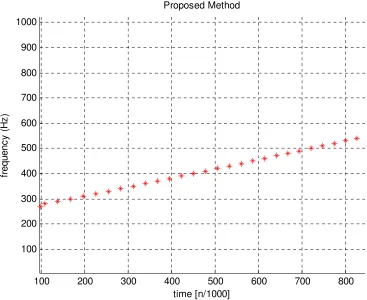
I. Test on single linear spectral component signal
The resulting projection curve shown in Figure 23 is used to find at which time instance each basis
function provides the highest peak. As a reminder, each basis function is a cosine or sine segments.
Therefore, if a basis function provides a high peak at a particular instance, it is implied that the
instantaneous frequency at that point in time is similar to that at the projected cosine/sine. Peak
detection is applied to search for highest matching frequencies. If more than one peak with high
amplitude is found at the same time instance by projecting different basis functions, the signal is
determined to have multiple components. Then a multi-peak detection combined with tracking
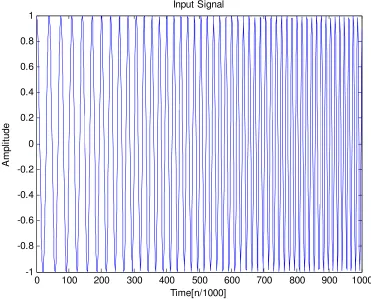
algorithm is necessary to find each component in the signal. The test signal in Figure 20 has only
one component which results in only one peak being detected. However, the plot of the
reconstructed spectral trajectory appeared to be non-continuous because of the use of a scanning
interval of 10Hz. The use of frequency scanning intervals reduces a tremendous amount of
computations needed for detecting chirps but also degrades the frequency resolution on the
time-frequency plane. As a result, when computing resources are scarce, increasing the time-frequency
scanning intervals provides a clear advantage. However, the designer must be cautioned that only
when chirps are linear and slowly changed, large intervals are appropriate. Otherwise, when chirps
are fast changing, either line regression or smaller scanning interval must be used to maintain
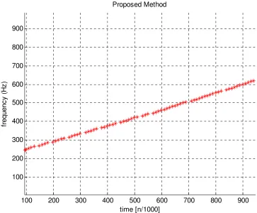
Figure 25 illustrates the result from the same signal but with smaller frequency scanning intervals
and larger time interval τ. The detected points are obviously denser when using small search
frequency intervals. Both figures, however, display very consistent results, a straight line with
slope of 0.001 starting at 200 Hz. Result from Figure 24 is obtained with a smaller window size
(parameter k) of 4 times the period of the searching frequency i versus 10 times as in Figure 24.
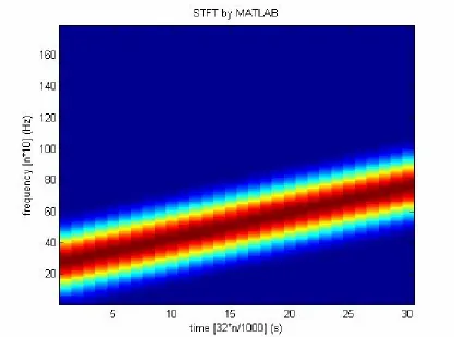
Finally, the results are compared against STFT with an FFT size of 1024 which produces a similar
curve to the proposed method’s result. The result from the STFT is obtained by using MATLAB
which produces an image-type plot. Because of its high resolution in time scale, the time-frequency
0 100 200 300 400 500 600 700 800 900 1000 -1
-0.8 -0.6 -0.4 -0.2 0 0.2 0.4 0.6 0.8 1
Input Signal
Time[n/1000]
A
m
p
lit
u
d
e
0 50 100 150 200 250 300 -1
-0.8 -0.6 -0.4 -0.2 0 0.2 0.4 0.6 0.8 1
Cosine Segment
Time [n/1000]
A
m
p
lit
u
d
e
0 50 100 150 200 250 300 -1
-0.8 -0.6 -0.4 -0.2 0 0.2 0.4 0.6 0.8 1
Sine Segment
Time [n/1000]
A
m
p
lit
u
d
e
0 100 200 300 400 500 600 700 800 900 1000 0
0.1 0.2 0.3 0.4 0.5 0.6 0.7
Signal Resulting from Projection
Time [n/1000]
A
m
p
lit
u
d
e
100 200 300 400 500 600 700 800 100
200 300 400 500 600 700 800 900 1000
fr
e
q
u
e
n
c
y
(
H
z
)
time [n/1000] Proposed Method
Figure 24: Results from Proposed Method with Peak Detection (Window Size = 10*Period of i, τ = 1
100 200 300 400 500 600 700 800 900 100
200 300 400 500 600 700 800 900
fr
e
q
u
e
n
c
y
(
H
z
)
time [n/1000] Proposed Method
Figure 25: Results from Proposed Method with Peak Detection (Window Size = 4*Period of i, τ = 10
Figure 26: Results from STFT (Spectrogram) by MATLAB (Window Size = 64, FFT size = 1024, 50% overlapped)
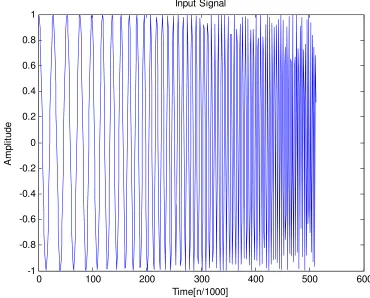
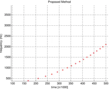
II. Test on single non-linear spectral component signal
In this test, a quadratic chirp is generated starting at 300Hz. Applying the proposed method, a
smooth and accurate trajectory is detected and reconstructed in both cases of using large frequency
interval (100Hz) and small frequency interval (5Hz). The result from using small frequency
interval, however, is smoother due to the higher frequency resolution. On the other hand, STFT’s
trajectory is not smooth in the case of using large window size (64 samples) and 50% overlapping.
The trajectory is smoother when using small window size (32 samples) and 100% overlapping.
0 100 200 300 400 500 600 -1
-0.8 -0.6 -0.4 -0.2 0 0.2 0.4 0.6 0.8 1
Input Signal
Time[n/1000]
A
m
p
lit
u
d
e
100 150 200 250 300 350 400 450 500 500
1000 1500 2000 2500 3000 3500
fr
e
q
u
e
n
c
y
(
H
z
)
time [n/1000] Proposed Method
100 150 200 250 300 350 400 450 500
1000 1500 2000 2500 3000 3500
fr
e
q
u
e
n
c
y
(
H
z
)
time [n/1000] Proposed Method
Figure 29: Results from Proposed Method with Peak Detection (Window Size = 4*Period of i, τ = 10,
Figure 31: Results from STFT (Spectrogram) by MATLAB (Window Size = 32, FFT size = 1024, Overlapped Size = 30)
III. Test on single non-linear fast-changing spectral component signal
In this test case, the signal is generated with quadratic chirp rate that is twice as fast as the previous
case (0.00002). The time shift parameter τ of the proposed method is varied to demonstrate its
effects on the results. Figure 37 is the result from STFT which shows an almost linear trajectory.
Figure 34 and Figure 35 are results from proposed method with a time shift of 10 samples in both
cases. However, in Figure 33, only the cosine part of (20) is used which leads to non-continuous
trajectory. In Figure 34, trajectory resulted from using widow sizes that are 4 times the projecting
Figure 33 also shows that trajectory resulted from using 100Hz interval scanning frequency is
more un-continuous. Consequently, when computing resources are limited, to maintain reasonable
accuracy, the most important consideration should be to increase the time-shift parameter τ to
reduce computational time.
0 100 200 300 400 500 600 -1
-0.8 -0.6 -0.4 -0.2 0 0.2 0.4 0.6 0.8 1
Input Signal
Time[n/1000]
A
m
p
lit
u
d
e
100 150 200 250 300 350 400 450 500 500
1000 1500 2000 2500 3000 3500
fr
e
q
u
e
n
c
y
(
H
z
)
time [n/1000] Proposed Method
100 150 200 250 300 350 400 450 500 500
1000 1500 2000 2500 3000 3500
fr
e
q
u
e
n
c
y
(
H
z
)
time [n/1000] Proposed Method
Figure 34: Results from Proposed Method with Peak Detection (Window Size = 4*Period of i, τ = 10,
100 150 200 250 300 350 400 450 500 1000
1500 2000 2500 3000 3500
fr
e
q
u
e
n
c
y
(
H
z
)
time [n/1000] Proposed Method
Figure 35: Results from Proposed Method with Peak Detection (Window Size = 4*Period of i, τ = 10,
100 150 200 250 300 350 400 450 500 500
1000 1500 2000 2500 3000 3500
fr
e
q
u
e
n
c
y
(
H
z
)
time [n/1000] Proposed Method
Figure 36: Results from Proposed Method with Peak Detection (Window Size = 2*Period of i, τ = 10,
Figure 37: Results from STFT (Spectrogram) by MATLAB (Window Size = 100, FFT size = 1024, Overlapped Size = 50)
IV. Test on multiple linear spectral component signal
With multiple components crossing each other, the results from both STFT and the proposed
method produce similar trajectories. No spectral components are detected at time 0.03s using the
0 100 200 300 400 500 600 700 800 900 1000 -2
-1.5 -1 -0.5 0 0.5 1 1.5 2
Input Signal
Time[n/1000]
A
m
p
lit
u
d
e
200 300 400 500 600 700 800 900 500
1000 1500 2000 2500 3000 3500
fr
e
q
u
e
n
c
y
(
H
z
)
time [n/1000] Proposed Method
Figure 40: Results from STFT (Spectrogram) by MATLAB (Window Size = 64, FFT size = 1024, Overlapped Size = 32)
V. Test on multiple linear non-crossing spectral component signal
For linear chirping with both components chirping non-crossing (non-destructive) to each other,
both STFT and the proposed method produce similar trajectories. The proposed method is able to
0 100 200 300 400 500 600 700 800 900 1000 -2
-1.5 -1 -0.5 0 0.5 1 1.5 2
Input Signal
Time[n/1000]
A
m
p
lit
u
d
e
200 300 400 500 600 700 800 900 1000
1500 2000 2500 3000 3500
fr
e
q
u
e
n
c
y
(
H
z
)
time [n/1000] Proposed Method
Figure 43: Results from STFT (Spectrogram) by MATLAB (Window Size = 64, FFT size = 1024, Overlapped Size = 32)
VI. Test on multiple linear and quadratic spectral component signal
In this test case, a linear and a quadratic chirp are combined. Aliasing is purposefully allowed to
occur at approximately 0.45s which produces a fast downward chirp component (Figure 44). The
proposed method performs acceptable for linear and quadratic chirp in this case. Figure 44 also
shows the input signal in the time domain with almost zero-amplitude approximately at time
0.015s because the two signal components add destructively. This is the reason why there is almost
this time because of the fact that the two components are too close together which make peak
detection very difficult. Both window sizes used for the STFT are no able to produce acceptable
results. This emphasizes the fact that an appropriate STFT window may not be easy to find. Figure
46 displays the results of STFT when using a window size that is too small (16 samples) which is
barely acceptable for the quadratic component but is unacceptable for the linear component. On the
other hand, Figure 47 is the result of using window size that is too large (128) which produces
acceptable result for the linear component but unacceptable result for the quadratic component. In
practice, therefore, it is difficult to estimate the optimum window size in the case of using STFT
unless an optimal size is iteratively selected after FT is done which needs more intensive
calculations. In contrast, the proposed method uses window sizes which are immensely
proportional to the searching frequencies. This implies that the window sizes adapt to the
frequencies of the particular basis used. Therefore, the trajectories for both components are visible
0 100 200 300 400 500 600 -2
-1.5 -1 -0.5 0 0.5 1 1.5 2
Input Signal
Time[n/1000]
A
m
p
lit
u
d
e
100 150 200 250 300 350 400 450 500 2000
3000 4000 5000 6000 7000
fr
e
q
u
e
n
c
y
(
H
z
)
time [n/1000] Proposed Method
Figure 46: Results from STFT (Spectrogram) by
Figure 47: Results from STFT (Spectrogram) by
CHAPTER 4
REAL-TIME HARDWARE IMPLEMENTATION
Because of the adaptability of the algorithm, it can be tailored to fit on a flash drive of a Digital
Signal Processing board and can produce meaningful result in real-time. In this paper, the Texas
Instrument C6713 Digital Signal Processing (DSP) board is chosen for testing and analyzing
generated signals which possess different spectral properties. The results are displayed in real-time
to illustrate how the proposed algorithm performs in practical applications. This board was chosen
because of its availability at the University of New Orleans and its popularity as a general Digital
Signal Processing (DSP) board in many practical applications. The board has a moderate
processing speed of about 200 MHz. However, with its memory space of 16MB and its sound
processing unit, which has both stereo inputs and outputs, it serves the intended purpose of testing
Figure 49: TMS320C6713 DSP Development Board (Image by Texas Instruments, Inc.)
I. DSP Board Specifications:
• TMS320C6713 Board features [11]:
• 512K Flash and 16MB SRAM for application binary and memory space
• Code Composer StudioTM Integrated Development Environment software (somewhat like
Visual Studio)
• USB communication to host computer
• +5V Power supply (with AC adapter)
• 24-bit stereo audio codec (with two input lines and two output lines)
• Eight 32-bit instructions/cycle
• 32/64- bit data word
• 225-, 200Mhz (GDP), and 200-, 167Mhz clock rates
• 4.4-, 5-, 6 Instruction cycle times
• 1800/1350, 1600/1200, and 1336/1000 MIPS/MFLOPS
• Two ALUs (fixed point)
• Four ALUs (floating and fixed point)
• 32-bit general purpose registers
• Instruction packing to reduce code size
• All instructions conditional
II. DSP code design and implementation
The Integrated Development Environment (IDE) software Code Composer Studio included in the
DSP kit is used for implementing and designing a test application for the proposed algorithm. The
IDE is a user-friendly interface that is similar to Visual Studio which eases the user in coding DSP
algorithms. Most of the board’s initialization and configuration are done with minimal user’s
efforts. For the test application, the code is developed in C++ language.
The board must be powered up and connect to the host computer which has Code Composer
Studio installed before starting Code Composer Studio. After loading the project file (*.pjt), the
Figure 50: Code Composer Studio Interface
The sampling rate and buffer size for the test application were selected as 8 kHz and 128 samples,
respectively. The application also is designed to use buffered pipe input/output in which a
queue-type buffer is provided by the IDE for importing and outputting sound data from the outside world.
Since buffer pipe is used, the applications files will have the names beginning with pip_audio.
Sampling rate and buffer size settings can be set by changing the properties of the file
Figure 51: Setting the Number of Samples per Buffer Size
The sampling frequency can be set to 8 KHz by modifying the file “pip_audio.c,” the main source
file for this project.
These lines must be placed after the “include” statements and before initializing at the input/output
DSP sound. The sampling frequency can be changed to any value of 8, 32, 44, 48, and 96 KHz. #ifdef AIC23_REG8_DEFAULT
#undef AIC23_REG8_DEFAULT
Since the input and output buffers and any filters coefficient used are floating-point variables and
very large in size, these variables must be put in extended memory, SRAM, so that the remaining
program code can fit on the flash drive space. The following steps need to be done in order to place
those data arrays in extended memory.
Append the following lines at the end of the file pip_audio.cmd to define a new section in
extended memory. In Code Composer Studio, the files that are ended with extension .cmd are
called linker files. These files organize program code in memory and link various modules and/or
libraries that the main program needs in order to run successfully.
In the main application file, pip_audio.cmd, for each data array that needed to be in extended
memory, the following statements are placed after the data is defined. SECTIONS
{
.EXTRAM :> SRAM
These statements align the data array on float-size boundary, which is necessary for some filtering
operations and place the array on .EXTRAM as defined earlier.
The test application uses DSP/BIOS to schedule real-time processing and displaying the results.
DSP/BIOS is a scalable real-time kernel. It provides preemptive multi-threading, hardware
abstraction, and real-time analysis. A test signal is generated while the processing is being done for
more efficient testing. To apply projection of coefficient segments on the test signal, a library
Texas Instruments (TI) function, called DSPF_sp_dotprod, is used. The name stands for
single-precision dot product. TI provides a “hand made” library that contains a DSP function coded in
Assembly language by design engineers for each particular DSP board to provide the users with
the fastest and most efficient way of utilizing the DSP processors. In order to use this function, the
library file “dsp67x.lib” is added to the project’s environment and the header file, so that the
function is included at the beginning of the main test application code: float out[B_SIZE] = {0.0}; // output buffer with size=B_SIZE
#pragma DATA_ALIGN(out, sizeof(float))
#pragma DATA_SECTION(out,”.EXTRAM”)
![Figure 19: Spectrogram of results obtained with Chirplet Based Adaptive Approximation (5 chirplets) (Image by Qian and Chen) [9]](https://thumb-us.123doks.com/thumbv2/123dok_us/8934124.1847392/32.612.176.445.70.376/figure-spectrogram-results-obtained-chirplet-adaptive-approximation-chirplets.webp)