Optimal control of an HIV model

________________

*_{Corresponding author}

Received November 20, 2015

461

OPTIMAL CONTROL OF AN HIV MODEL

OGBAN GABRIEL IYAM*_{, LEBEDEV KONSTANTIN ANDREYEVICH}

Department of Computational Mathematics and Informatics, Kuban State University, Krasnodar, Russia

Copyright © 2016 Iyam and Andreyevich. This is an open access article distributed under the Creative Commons Attribution License, which permits unrestricted use, distribution, and reproduction in any medium, provided the original work is properly cited.

Abstract: In this article we propose an optimal control problem, a drug regimen that inhibits the rate at which the uninfected cells become infected, inhibits the influx of the virus from the external lymphoid compartment and at the same time minimizing the drug cost. The model considered here has a different interpretation of the effects of treatment, since the production of virus from the external lymphoid compartment is not immediately blocked by treatment and thus influences the viral decay rate. The model utilizes a system of ordinary differential equations which describes the interaction of the immune system with the human immunodeficiency virus (HIV). The optimal control problem is transferred into a modified problem in measure space, one in which existence of the solution is guaranteed by compactness of space. By an approximation, we obtain a finite dimensional linear programming problem which gives an approximate solution to the original problem. Our numerical solutions obtained with the help of MATHCAD shows treatment protocols which could maximize the survival time of patients in the short and long term process. Simulations are given with the treatment parameter corresponding to suppression of virus influx from the lymphoid compartment.

Keywords: HIV model; CD T4 _cell; _{treatment; optimal control; linear programming; simulation; measure theory;}

approximate solution; drug; MATHCAD.

2010 AMS Subject Classification: 97M10.

1. Introduction.

Since it was first detected about 30 years ago, AIDS - Acquired Immunodeficiency

Syndrome as a disease has continued to affect the whole world. It is caused by Human

Immunodeficiency Virus (HIV). According to WHO, of the 35 million people worldwide living

with HIV infection today, more than 24 million are in low- and middle- income countries,

particularly in sub-Saharan Africa [15].

Even though there have been advances in our scientific understanding of HIV and its

prevention and treatment as well as years of significant effort by the global health community

and leading government including civil society organizations, most people living with HIV or at

risk for HIV do not have access to prevention, care, and treatment, and there is still no absolute

cure. However, effective treatment with antiretroviral drugs can control the virus so that people

with HIV can enjoy healthy lives and reduce the risk of transmitting the virus to others.

Once HIV infects the body, its target is CD4+Tcells, which are an important part of the

human immune system. The infected cells produce a large number of new viruses. Highly active

antiretroviral therapy (HAART) enables effective suppression of HIV-infected individuals and

goes a long way to prolonging the time before the onset of acquired immune deficiency

syndrome (AIDS). This could be for years or even decades and, therefore, increases life J. Math. Comput. Sci. 6 (2016), No. 3, 461-472

expectancy and quality to the patient. However, because of the long-lived infected cells and sites

within the body where drugs may not achieve effective levels of penetration, antiretroviral

therapy cannot eradicate HIV from infected patients [1]. Reverse transcriptase inhibitors (RTI)

and Protease inhibitor (PI) are the two major constituents of HAART. RTIs act by preventing

HIV from infecting cells by blocking the integration of the HIV viral code into the host cell

genome while protease inhibitors prevent infected cells from replication of infectious virus

particles, this enables it to reduce and maintain viral load below the limit of detection in many

patients.

Until date, many of the host-pathogen interaction mechanisms during HIV infection and

progression to AIDS remain unknown. Mathematical modeling of HIV infection is of interest

since there are no adequate animal models to test the efficacy of drug regimes. These models

provide the essential tool to capture a set of assumptions and provide new insights into questions

that are difficult to answer by clinical or experimental studies. To describe various aspects of the

interaction between the human immune system and HIV, a number of mathematical models have

been formulated. For instance, modeling of the kinetics of HIV RNA under drug therapy has led

to substantial insight into the dynamics and pathogenesis of HIV [14, 6, 16] and the existence of

multiple reservoirs that have made eradication of the virus difficult. Wodaz and Nowak [10]

presented the basic model of HIV infection, which contains three state variables: healthy CD4+

T-cells, infected CD4+ T-cells, and concentration of free virus. This model which has been

modified offers important theoretical insights into the immune control of the virus, based on

treatment strategies, while maintaining a simple structure [9].

In the first section of this article, a mathematical model of HIV dynamics that includes

the effect of two treatments and analysis of optimal control is carried out with regards to

appropriate goals.

The remaining part of this paper is organized as follows: in Section 2, the underlying HIV

mathematical model is described with an increase phase space, Section 3 describes the

formulation of the control problem. In section 4, we attempt to approximate the obtained optimal

control problem by a linear programming problem. Numerical results using MATHCAD is the

subject of Section 5. Section 6 is the conclusion.

2. Statement of the model

We consider a system of ordinary differential equation (ODE) presented by Kirschner and

Webb [7] and used by Pritikin [4] which describes the interaction between HIV and the immune

system of the body. In this model,

T

(

t

)

represents the uninfected

CD

4



T



cell

population at

the time

t

,

T

_S

(t

)

represents the drug-sensitive infected

CD

4



T



cell

population at time t,

)

(t

T

_r represents the drug-resistant CD4+T-cell population at time t,

V

_S

(t

)

represents the

drug-sensitive virus population at time t, and

V

r

(t

)

represent the drug resistant virus population at

time t and

V

(

t

)



V

_S

(

t

)



V

_r

(

t

)

represent the total virus population at time t. All these

populations are measured in the blood plasma, which constitutes only 2% of their total, the rest

) ( )) ( ) ( ) ( ( ) ( ) ( ) ( ) ( ) ( ) ( 1

1 t T t V t t KV t KV t T t l t mT t S dt t dT r r s s    

  (2.1)

)

(

)

(

)

(

)

(

)

(

)

(

)

(

)

(

2 1

1

t

K

V

t

T

t

m

T

t

l

t

T

t

V

t

dt

t

dT

s s s s

s









_(2.2)

)

(

)

(

)

(

)

(

)

(

)

(

)

(

2

1

T

t

l

t

T

t

V

t

m

t

T

t

V

K

dt

t

dT

r r r r

r







_(2.3)

) ( ) ( ) ( ) ( ) ( ) ( ) 1 ( ) ( 2

3T t V t K T t V t t G t

l q dt t dV s s v s

s    



_(2.4)

) ( ) ( ) ( ) ( ) ( ) ( ) ( ) ( ) ( ) ( 3 3 t V B t V V G t V t T k t V t T q t V t T l dt t dV _r r r V S r r    





(2.5)

with given initial values.

The definitions and numerical values of the constants of equations (2.1) - (2.5) are listed

in Table 1 [11, see Ogban and Lebedev]. They are as used for the model without treatment.

In these equations, treatment is modeled by the decreasing functions



₁

(

t

)

and



₂

(

t

)

.

The function



₁

(

t

)

inhibits the rate at which uninfected

CD

4



T

cells become infected and

)

(

2

t



inhibits the influx of virus from the external lymphoid compartment). The parameters

2 1

,

c

c

and

c

₃ control the speed and strength of the drug-induced inhibitions). It is assumed that

the functions



₁

(

t

)

and



2

(

t

)

are determined by the expressions

)

(

exp(

)

(

_{1 0}

1

t





c

t



t



(2.6)

)}

),

(

max{exp(

)

(

_{2 0 3}

2

t





c

t



t

c



3. Optimal control formulation

In this section, we formulate an optimal control problem in accordance with the

recommendations developed by the committee of the international society for AIDS [2]. The

committee in its recommendations pointed to the possibility of increasing the effectiveness of

treatment by a strong combination of antiretroviral drugs. The model (2.4) -(2.6) meets this by

the consideration of treatment with two different mechanisms of action. It is further reflected in

the optimization problem by the introduction of two control variables. In particular, during

medication, the dynamics of the source function is given as

),

(

)

(

1 1 1 1

t

c

f

dt

t

d





trt







1

)

0

(

1





(3.1)

),

(

)

(

2 2 2

2

_f

_c

_t

dt

t

d





trt









₂

(

0

)



1

(3.2)

We note that the second of the equation of (2.6) defined by the maximum does not meet

the objective function of continuity and smoothness. To achieve this,



2

(

t

)

is written as

]

)

(

[

1

)

(

3 2 3 2 2 2

c

t

c

c

f

dt

t

d

ntctrt













,



₂

(

0

)



1

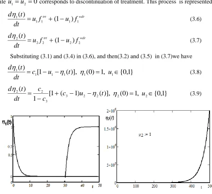
(3.3)

Figure 1. Graph of dynamics model of control functions with constant treatment

We write the growth equations for the modified functions at intervals of drug withdrawal

as

)]

(

1

[

)

(

1 1 1

1

t

c

f

dt

t

d





wdr







(3.4)

)]

(

1

[

1

)

(

2 3

2 2

2

t

c

c

f

dt

t

d



wdr











(3.5)

Control variables, that is switches

u

₁ and

u

₂ are introduced and embedded into the

treatment functions as follows:

u

₁



u

₂



1

corresponds to the process of treatment being on

while

u

₁



u

₂



0

corresponds to discontinuation of treatment. This process is represented as

wdr trt

f

u

f

u

dt

t

d

1 1 1

1 1

)

1

(

)

(









(3.6)

wdr trt

f

u

f

u

dt

t

d

2 2 2

2 2

)

1

(

)

(

_

_

_



(3.7)

Substituting (3.1) and (3.4) in (3.6), and then(3.2) and (3.5) in (3.7)we have

)],

(

1

[

)

(

1 1 1

1

_c

_u

_t

dt

t

d



_









₁

(

0

)



1

,

u

1



{

0

,

1

}

(3.8)

)],

(

)

1

(

1

[

1

)

(

2 2 3

3 2 2

t

u

c

c

c

dt

t

d



_

_

_

_







₂

(

0

)



1

,

u

₂



{

0

,

1

}

(3.9)

Figure 2. Dynamics of model showing structured treatment.

Thus, the system of differential equations(2.1)-(2.5) together with the controls is written

as

)

(

))

(

)

(

)

(

(

)

(

)

(

)

(

)

(

)

(

)

(

1

1

t

T

t

V

t

t

K

V

t

K

V

t

T

t

l

t

mT

t

S

dt

t

dT

r r s

s









)

(

)

(

)

(

)

(

)

(

)

(

)

(

)

(

2 1

1

t

K

V

t

T

t

m

T

t

l

t

T

t

V

t

dt

t

dT

s s s s

s









)

(

)

(

)

(

)

(

)

(

)

(

)

(

2

1

T

t

l

t

T

t

V

t

m

t

T

t

V

K

dt

t

dT

r r r r

r







)

(

)

(

)

(

)

(

)

(

)

(

)

1

(

)

(

2

3

T

t

V

t

K

T

t

V

t

t

G

t

l

q

dt

t

dV

s s v s

s











(3.10)

)

(

)

(

)

(

)

(

)

(

)

(

)

(

)

(

)

(

)

(

3 3

t

V

B

t

V

V

G

t

V

t

T

K

t

V

t

T

ql

t

V

t

T

l

dt

t

dV

_r r r v s r r











)]

(

1

[

)

(

1 1 1 1

t

u

c

dt

t

d



_

_

_

_

)]

(

)

1

(

1

[

1

)

(

2 2 3 3 2

2

_c

_u

_t

c

c

dt

t

d



_











This paper aims to propose a drug regimen that inhibits the rate at which the uninfected

cells become infected and inhibits the influx of the virus from the external lymphoid

compartment at the same time minimizing the drug cost. This can be modeled as follows. The

main purpose of treatment is to prolong the life of a patient. There are three categories of disease

severity which is determined by the level of concentration of

CD

4



T



cell

present in the blood:

(i) greater than

500

unit

/

mm

3

(ii) 200



T



500

(iii) <200

The third category of patients develops the disease that is known as acquired

immunodeficiency syndrome AIDS. The lower value of the concentration of T cells is a natural

boundary of the studied processes in the immune system. This means that the phase space of the

system (4.10) should consider its trajectory ending on the hypersurface

0

)

(

t



T

*



T

(3.11)

Here,

T

* - some constant (for example,

T

*



500

units

/

mm

3 or

3 *

/

200

units

mm

T



). The task of extending the life of the patient is that the immune system

had reached the borders of (4.15) as late as possible.

Assume that at the beginning of treatment

*

)

(

t

T

T



,

t



[

t

0

,

t

f

],

T

(

t

)



T

*

_(3.12)

A problem arising from the use of most chemotherapies is the multiple and sometimes

harmful side effects as well as the ineffectiveness of treatment after a time due to the capability

of the virus to mutate and become resistant to the treatment. Global effects of this phenomenon

are considered by imposing limited treatment interval in line with the recommendations in [2],

that is the treatment last for a given period of time

t

₀ to

t

₀





. Therefore, the treatment interval

must contain the control function

u

_i

(.)

Here, we follow [8] in assuming that the cost of the treatment is proportional to

u

2

(

t

)

at

time

t

.

Therefore the overall cost of treatment is



f

t

t

dt

t

u

0

)

(

2

. So the following functional should

be maximized:







f

t

t f

f

u

t

u

t

dt

t

0

)

(

)

,

(



2



. (3.14)

The relative importance of maximizing the survival time

t

_f and minimizing the systemic

cost to the body necessitate the use of the parameter



.

The system of differential equations (3.10) can be represented in the generalized form as

)

),

(

),

(

(

)

(

t

g

x

t

u

t

t

x





,

x

(

0

)



0

.

( 3.15 )

Assume that

U

denotes the set of all measurable control functions

u

(.)



[

0

,

1

],

where

(.)

u

satisfies (3.13), and the corresponding solution of (3.15) at final time

t

_f satisfies [3.12].

Therefore, we are seeking for

u

*

(.)



U

such that

)

,

(

)

,

(

* *

u

t

u

t

f



f





,



u



U

, (3.16)

Setting

(

(

),

(

),

)

1

2

(

),

0

x

t

u

t

t

u

t

f







then the optimal drug regimen problem, while

ignoring

t

₀, can be represented as





f

f

t

t k u

t

f

x

t

u

t

t

dt

0

)

),

(

),

(

(

max

0

, (3.17)

Subject to

)

),

(

),

(

(

x

t

u

t

t

g

x





(3.18)

,

)

(

t

₀

x

₀

x



T

(

t

_f

)



CD

4

_crit, (3.19)





CD

crit

t

T

(

)

4

,

t



[

t

0

,

t

f

],

(3.20)

This is an optimal control problem (OCP). The set

U

may be empty. If

U

is not empty,

then the function measuring the performance of the system may not achieve its maximum in the

set

U

. In order to overcome these difficulties, in the next section, we transfer the modified

problem in measure space.

4. Approximation of OCP by Linear Programming Problem

We now use measure theory for solving optimal control problems based on the idea of

Young [3] and applied by Rubio [5]. This method has been extended for approximating the time

optimal problems by a Linear programming model [13].

4.1 We assume that the state variables

x

(.)

and the control variables

u

(.)

, respectively

get their values in the compact sets

B



B

₁

*

B

₂

*

...

B

₇



R

7 and

U



R

.

By setting

]

,

[

t

0

t

f

J



, we derive weak forms for (3.18) - (3.20).

Definition 1. A trajectory pair

p



[

x

(

t

),

u

(

t

),

t

)]

is said to be admissible if the

(i)

x

(.)



A



t



J

and is absolutely continuous.

(ii)

u

(.)



U



t



J

and is measurable on

J

.

(iii)

p

satisfies (3.18)-(3.20) everywhere on

J

0

We assume that the set of all admissible triples is nonempty and denote it by

H

.

Let

p

be an admissible triple,

B

an open ball in

R

8 containing

J

*

A

,

and let

C



(B

)

be the space of

all real-valued continuous differentiable functions on it. Let





C



(

B

)

and define



g as follow:

)

),

(

(

)

),

(

),

(

(

).

),

(

(

)

),

(

),

(

(

x

t

u

t

t

x

x

t

t

g

x

t

u

t

t

t

x

t

t

g











(4.1.1)

for each

[

x

(

t

),

u

(

t

),

t

]





,

where





J

*

A

*

U

.

The function



g is in the space of

),

(



C

the set of all continuous functions on the compact set



. Since

p



[

x

,

u

,

t

f

]

is an

admissible triple, we have



f





f



t

t

t

t

t x

g

dt

t

t

x

t

x

t

t

x

dt

t

t

t

u

0 0

)

),

(

(

)

(

).

),

(

(

)

),

(

),

(

(

























(

x

(

t

f

),

t

f

)

(

x

(

t

0

),

t

0

)

(4.2)

for all





C



(B

).

Let

(

0

)

J

D

be the space of all infinitely differentiable real-valued

functions with compact support in

J

0. Define

),

(

)

),

(

),

(

(

)

(

)

(

)

),

(

),

(

(

x

t

u

t

t

x

n

t

t

g

n

x

t

u

t

t

t

n













)

(

,

7

,...,

2

,

1

0

J

D

n









_(4.1.3))

Since

p



[

x

,

u

,

t

_f

]

is an admissible triple, then the function



(.)

has compact support

in

J

0,



(

t

0

)





(

t

f

)



0

.

Thus for

n



1

,

2

,...

7

,

and for all

(

),

0

J

D





from (4.3) and using

integration by parts, we have



f





f







f



t

t

t

t

t

t n n

n

dt

t

t

t

u

t

x

g

dt

t

t

x

dt

t

t

u

t

x

0 0 0

0

)

(

)

),

(

),

(

(

)

(

)

(

)

),

(

),

(

(







(4.1.4)

Also by choosing the functions which are dependent on time only, we have



f



t

t

dt

t

t

u

t

x

0

)

),

(

),

(

(



_









C



(



),

(4.1.5)

where

C



(



)

is the space of all function in

C

(



)

that depend only on time and



_ is

the integral of



(.)

on

J

.

Equations (4.2),(4.4) and (4.5) are the weak forms of (3.18)-(3.20).

Remark: The constraints (3.19) are considered on the right-hand side of (4.2) by choosing

suitable functions





C



(B

)

which are monomials of

T

(

t

)

. More so, the constant (3.20) is

considered, by choosing an appropriate set

A

.

Again by considering the mapping







J

p

:

L

L

(

x

(

t

),

u

(

t

),

t

)

dt

,



L



C

(



)

(4.1.6)

we note it is positive linear functional on

C

(



)

and we can construct a 1-1

p

p





of admissible triples in

H

into the linear mapping



_p.

Consequently, from (4.1.2), (4.1.4) and (4.1.5), we can conclude that maximizing the

functional (3.17) over admissible space

H

, changes to the following optimization problem in

functional space:

)

(

max

p

f

0

H

p



(4.1.7)

Subject to

,

)

(











g

p





C



(B

)

(4.1.8)

0

)

(





n

p



n



1

,

2

,...,

7

,

(

),

0

J

D





(4.1.9)

,

)

(











_p





C

1

(



)

(4.1.10)

4.2 Measure space. Let

M



(



)

denote the space of all positive Radon measures on



.

By the Riesz representation theorem [12], there exists a unique positive Radon measure







such that







J

p

(

L

)

L

(

x

(

t

),

u

(

t

),

t

)

dt









L

(

x

(

t

),

u

(

t

),

t

)

d





(

L

),

L



C

(



).

(4.2.1)

Thus, we may change the functional space of the optimization problem to measure space.

This implies that the optimization problem (4.1.7)-(4.1.10) can be converted to the following

optimization problem in measure space:

)

(

max

₀

)

(

f

M



   (4.2.2)

Subject to

,

)

(







g









C



(B

),

(4.2.3)

,

0

)

(



n





1

,

2

,...,

7

,

(

0

),

J

D

n







(4.2.4)

,

)

(





_







1

(



),

C



(4.2.5)

We now define

Q

to be the set of all measure in

M



(



)

that satisfy (4.2.3)-(4.2.5) and

then we can show that there exists an optimal measure



* in

Q

where the point may be studied

without imposing conditions such as convexity. Formally, we state as follow:

Define the function

I

:

Q



R

as

I

(



)





(

f

₀

)

.

Theorem. The measure theoretical problem of maximizing (4.2.2)-(4.2.5)has an optimal

solution say *

,

*

.

Q

where







Remarks: The above theorem guarantees the existence of an optimal solution.

Proof. See [ ] and note that the constraints (4.2.4) and (4.2.5) are special cases of (4.2.3).

This implies that the set

Q

can be written as

}.

)

(

:

)

(

{

) (























 

g B

C

M

Suppose that

p



[

x

,

u

,

t

f

]

is an admissible triple. Surely,

}

)

1

(

:

)

(

{





M









t

_f



t

₀ is compact in the weak topology. Moreover, the set

Q

as an

intersection of the closed singleton sets

{





}

under the continuous function







(



g

)

is

also closed. Hence,

Q

is a closed subset of a compact set. Since the functional I, mapping the

compact set Q on the real line is continuous and takes its maximum from Q the compactness is

proved.//

Obviously, the problem is an infinite dimensional linear programming problem, and all

the functions (4.2.2) - (4.2.5) are linear in



.

We obtain an approximate solution of this problem by the solution of a finite-dimensional linear program.

Proposition. If the linear program problem consisting of maximizing the function

I

over

the set

Q

_M of measures in

M



(



)

satisfies

,

)

(

g _i i











i



1

,...,

M

.

(4.2.7)

Then, Then,

J

I

J

I

Q Q

M

M

max

max







as

M





Proof. We have

Q



...



Q

_M



...

Q

₂



Q

₁, it follows, therefore, that

.

...

...

J

J

₂

J

₁

J





_M







The sequence

 

_

1

j j

J

is nonincreasing and bounded, so, it converges to a number



such

that





J

.

We show that





J

.

Set

R





_M1

Q

_M.Then

Q



R

and

max

I

.

R





It is

sufficient to show

Q



R

.

Assume





R

and





C



(B

).

Since the linear combination of

the function

{



j

,

j



1

,

2

,...}

is uniformly dense in

C



(B

),

there is a sequence

}



~

{

span

{



j

,

j



1

,

2

,

,

,

,

},

such that



K

~

_{tends to}

_

_{uniformly as}

_k

_

_

_.

_Thus,

3 2

1

,

S

,

S

S

tend to

zero as

k





where ₁

sup

|

~

|,

₂

sup

|

~

|,

t

x t K

K

x

S

S

















and

S

₃



sup

|







~

_k

|

.

Since





R

and the functional

f





(

f

)

is linear,

K g

K







₍

~

₎

_

_

~

_and







|

)

(

|





g



|

(

)

(

~

g

)

~

_K

|

K

g























)

~

(

)]}

,

(

~

)

,

(

[

)

,

,

(

)]

,

(

~

)

,

(

{[

_x

x

t

_K

x

t

g

x

u

t

_t

x

t

_kt

x

t

d

_k

x































_

















S

₁

g

(

x

,

u

,

t

)

d



S

₂

d



2

S

₃

.

_(4.2.8)

The right-hand side of the above inequality tends to zero as

k





,

and the left-hand

side is independent of

k

;

therefore



(



g

)







.

Thus,

R



Q

and





J

,

which implies

//

.

J





The right-hand side of the above inequality tends to zero as

k





,

ant the left-hand

side is independent of

k

;

therefore



(



g

)







.

Thus,

R



Q

and





J

,

which implies

//

.

J



Proposition 3. The measure



* in the set

Q

_Mat which the functional

I

attains its

minimum has the form

),

(

1

* *

*







M

j

j j



z





(4.2.9)

Where *



0

,

*





,

j

z



and



(

z

)

is unitary atomic measure with the support being the

singleton set

{

*

},

j

z

characterized by



(

z

)(

F

)



F

(

z

),

z





.

We, therefore, restrict ourselves to finding a measure in the form of (4.2.9) which

maximizes the functional

I

and satisfies in M number of constraints (4.2.3)-(4.2.5). Thus by

choosing the functions



_i

,

i



1

,

2

,...,

M

₁

,



_K

,

k



1

,...,

M

₂

,

and



_S

,

s



1

,...,

S

,

the infinite

dimensional problem (4.2.2)-(4.2.5) is approximated by the following finite dimensional

nonlinear programming problem:



   

M

j

j j

z

f

z

imize

j

j ₁

0 ,

0

(

)

max



 (4.2.10)

Subject to











M

j

j g i

j

z

i

M

1

1

,

,...,

1

,

)

(







(4.2.11)











M

j

j n K

j

z

k

M

n

1

2

,

1

,...,

7

,

,...,

1

,

0

)

(





(4.2.12)

S

s

b

z

M

j

j S

j

(

)

_S

,

1

,...,

1







 





(4.2.13)

where

M



M

₁



4

M

₂



S

.

Obviously, (4.2.10)-(4.2.10) is a nonlinear programming

problem with

2

M

unknowns:



_j and

z

_j,

j



1

,...,

M

.

We are interested in LP problem. The

following proposition enables us to approximate the nonlinear programming problem

(4.2.10)-(4.2.3) by a finite dimensional linear programming problem.

Proposition 4. Let



_N



{

y

₁

,

y

₂

,...,

y

_N

}

be a countable dense subset of



.

Given

,

0





a measure

v



M



(



)

can be found such that

,

(

)

(

f

₀





*

f

₀₎





v









)



(

)



(

_ig * _ig

v

,

i



1

,...,

M

₁

,

,

)

(

)

(







*



n





k n

k

v

k



1

,...,

M

₂

,

n



1

,

2

,...,

7

,

,

)

(

)

(







*







S S

v

s



1

,...,

S

,

(4.2.14)

where the measure

v

has the form







M

j

j j

y

v

1

*

),

(





(4.2.15)

And the coefficients



*j

,

j



1

,...,

M

,

are the same as optimal measure (4.2.9), and

Proof. Let us rename the functions

,

,

,

,

,

0

s

s

f

n

k g i





and



_S

'

s

sequentially as

.

1

,...

2

,

1

,

j



M



h

j Then, for

j



,...,

M



1

,

)

(

)

(

max

)]

(

)

(

[

)

(

*

, * *

1 1

* * *

i j i j j i i M

j M

i

i j i j i

j

h

z

h

y

h

z

h

y

h

v



























 







(4.2.16)

where the

h

_j

s

are continuous. Hence, by choosing

y

_i

,

i



1

,...,

M

,

sufficiently close to

*

i

z

, we have









_M

j j i

j i j j

i

h

z

h

y

1 * *

,

(

)

(

)

max





.//

J

is divided into

S

subintervals in order to construct a suitable set



_N as follows:

,

1

,

1

)

1

(

0

0



























S

T

s

t

S

T

s

t

J

S

s



1

,...,

S



1

,

J

S



[

t

0

,

t

f

),

(4.2.17)

where

t

₀ is a lower bound for the optimal time

t

_f.

Therefore, according to (4.2.15), the nonlinear programming problem (33)-(36) is

converted to the following linear programming problem:



 

M

j

j j

f

y

j ₁

0

0

(

)

max



 (4.2.18)

Subject to

,

)

(

1









N

j

i j

g i

j



y





i



1

,...,

M

1, (4.2.19)







N

j

j n k j

y

1

,

0

)

(





k



1

,...,

M

₂

,

n



1

,...,

7

,

(4.2.20)









N

j

j s

j

y

b

_s

s

S

1

.

,...,

1

,

)

(

_





(4.2.21)

Conclusion

In this paper, we proposed and constructed an optimal control problem. we considered a system

of differential equations as a dynamic system which describes the various aspects of the

interaction of HIV with the immune system. This control problem is a drug regimen that inhibits

the rate at which the uninfected cells become infected, inhibits the influx of the virus from the

external lymphoid compartment and at the same time minimizing the drug cost. A measure

theoretical method is used to solve the problem. The method is not iterative and as such initial

guess of the solution is not required. Numerical results with constant treatment are obtained.

Conflict of Interests

The authors declare that there is no conflict of interests.

Acknowledgments

The authors would like to thank the anonymous referee for his/her comments that helped to

REFERENCES

[1] A. Carr. Toxicity of antiretroviral therapy and implications of drug development // Nature Review Drug recovery, 2 (2003), 624-634.

[2] C. C. J. Carpenter, D. A Cooper, and et al Updated Recommendations of the International AIDS Society-USA Panel, (2000).

[3] C. Young. Calculus of Variation and Optimal control, Saunders Philadelphia, Pa, USA, (1969).

[4] D. A. Pritikin. Optimal control mathematical model of HIV infection. Thesis for the scientific degree of candidate of physical and mathematical sciences. Moscow, (2004).

[5] D. A. Wilson, and J. E. Rubio. Existence of the optimal controls for the diffusion equation, Journal of Optimization Theory and Applications, 1 (1977), 91-101.

[6] D. D. Ho, A. U. Neumann, et.al; Rapid turnover of plasma virions and CD4 lymphocytes in HIV-1 Infection. Nature, 373 (1995), 123-126.

[7] D. Kirschner, G.F. Webb. Resistance, Remission, and Qualitative Difference in HIV Chemotherapy // Emerging Infectious Diseases, 3 (1997), 273-283.6.

[8] D. Kirschner, S. Lenhart, and S. Serbin. Optimal Control of the chemotherapy of HIV infection: scheduling amounts and initiation of treatment // Journal of Mathematical Biology, 35 (1997), 775-792.

[9] D. Wodarz, and M. A. Nowak. Mathematical models of HIV pathogenesis and treatment // BioEssays, 24 (2002), 1178-1187.

[10] D. Wodarz.and M. A. Nowak, Specific therapy regimes could lead to long-term immunological control of HIV, Proceedings of the National Academy of Sciences of the United States of America, 96 ( 1999), 14464-14469.

[11] G. I. Ogban, K. A. Lebedev. Mathematical model of the Dynamics of HIV infection without treatment. Polythematic online scientific journal of Kuban State Agrarian University. 110 (2015), 1-17.

[12] H. H. Mehne, M.H. Farahi and A. V. Kamyad. MILP modeling of the time-optimal control problem in the case of multiple targets // Optimal Controls Applications and Methods, 2 (2006), 77-91.

[13] J. E. Rubio. Control and Optimization: The Linear Treatment of Non-Linear Problems, Manchester University Press, Manchester, UK, (1986).

[14] Perelson, A., Neumann A., Markowitz, M. et al HIV-1 Dynamics in vivo: clearance rate, infected cell lifespan, and viral generation time//Science, 271 (1996), 1582-1586.

[15] The global HIV/AIDS Statistics (https://www.aids.gov/hiv-aids-basics/hiv-aids-101/global-statistics) 2015 accessed on 16th July 2015