of peer-reviewed research and commentary in the population sciences published by the Max Planck Institute for Demographic Research Konrad-Zuse Str. 1, D-18057 Rostock · GERMANY www.demographic-research.org
DEMOGRAPHIC RESEARCH
VOLUME 11, ARTICLE 10, PAGES 263-304
PUBLISHED 03 DECEMBER 2004
www.demographic-research.org/Volumes/Vol11/10/
DOI: 10.4054/DemRes.2004.11.10
A Research Article
published in honor of Eugene A. Hammel
Computing Time-Varying
Sex-Age-Specific Rates of Marriage/Union
Formation and Dissolution in Family
Household Projection or Simulation
1 Introduction 264
2 Computing Age-Specific Rates of Marriage/Union Formation and Dissolution that are Consistent with the Projected Propensities in the One-Sex Life Course Simulation Model
267
3 Computing Time-Varying Sex-Age-Specific Rates of Marriage/Union Formation and Dissolution that are Consistent with the Two-Sex Constraints and Projected Summary Measures in the Family Household Projection Model
273
3.1 Two alternative groups of summary measures of marriage/union formation and dissolution
274
3.1.1 General rates of marriage/union formation and dissolution 274 3.1.2 Overall propensities of marriage/union formation and
dissolution in the context of the period life table
275
3.1.3 Rationale, assumptions, and implications of the summary measures
277
3.2 Procedure for computing sex-age-specific rates which are consistent with the two-sex constraints and the projected summary measures
280
4 Concluding Remarks 284
5 Acknowledgements 286
Notes 287
References 291
Appendix A: Illustrative Numerical Applications to Verify the Convergence of the Iterative Procedure for Computing Age-Specific Rates of Marriage/Union Formation and Dissolution that are Consistent with the Projected Propensities in the One-sex Life Course Simulation model
295
Appendix B: Procedure for Computing Sex-Age-Specific Rates which are Consistent with the Two-Sex Constraints
A Research Article
published in honor of Eugene A. Hammel
Computing Time-Varying Sex-Age-Specific Rates of
Marriage/Union Formation and Dissolution in Family Household
Projection or Simulation
Zeng Yi 1 Eric Stallard 2 Zhenglian Wang 3
Abstract
This article presents two procedures that are useful in both macro and micro projection/simulation models concerning marriage/union formation and dissolution. One is for computing time-varying sex-age-specific rates that are consistent with independently projected life course propensities of marriage/union formation and dissolution in the one-sex life course simulation model. Another one is for computing time-varying sex-age-specific rates that are consistent with the two-sex constraints and with independently projected summary measures of marriage/union formation and dissolution in the two-sex family household projection model. Illustrative numerical examples based on U.S. data demonstrate that the proposed procedures are valid.
1 Zeng Yi is Research Professor at the Center for Demographic Studies and the Department of Sociology of Duke University ([email protected]), Professor of China Center for Economic Research at Peking University, and Distinguished Research Scholar at the Max Planck Institute for Demographic Research.
2 Eric Stallard is Research Professor and Associate Director of the Center for Demographic Studies at Duke University.
1. Introduction
The aims of this article are twofold: (1) to present a procedure for computing in the one-sex life course simulation model the time-varying one-sex-age-specific rates (output), which are consistent with independently projected life course propensities of marriage/union formation and dissolution (input), and with age-specific standard schedules as part of the input; and (2) to present another procedure in the two-sex family household projection model for computing the time-varying sex-age-specific rates (output), which are consistent with the two-sex constraints and with independently projected summary measures of marriage/union formation and dissolution (input), also with age-specific standard schedules as part of the input. The two procedures are presented, discussed, and numerically illustrated in the second and the third sections of this article.
In this section, we first discuss practical applications of family household projections and simulations with time-varying sex-age-specific demographic rates; we then discuss the reasons why new technical procedures are needed in computing sex-age-specific rates of marriage/union formation and dissolution in family household projections and life course simulations, in contrast to the classic population projection; and we present our modeling framework which includes marital statuses, cohabitation, and their combinations.
Family household projections and life course simulations with time-varying sex-age-specific demographic rates are useful in socio-economic, actuarial, welfare planning, policy analysis, and market trend studies. For example, welfare programs in the United States typically restrict eligibility to single-parent families (Yelowitz, 1998). As a result, projections of the costs of such programs depend heavily upon projections of the future numbers, types, and sizes of single-parent family households (Moffitt, 2000). Similar projections could characterize implied changes in Chinese family household structure and family support for the elderly in the next several decades if fertility and mortality rates continued to decrease to very low levels, while divorce rates increased substantially. Family household projections with time-varying sex-age-specific demographic rates would be highly responsive to these kinds of policy analysis concerns (Hammel et al., 1991; Zeng, Vaupel, and Wang, 1997, 1998; Zeng, Land, Wang, and Gu, 2004).
consumption, would imply larger aggregate demands for resources (Keilman, 2003) and would pose serious challenges to biodiversity conservation (Liu et al., 2003).
Family household projections with changing demographic rates could also be useful in consumption and market analyses for housing and consumer durables (such as automobiles, appliances, furniture, water, gas, and electricity), in the development of household related public utilities and services, and in the determination of long-term care needs for the elderly.
Household projections are among statistical offices’ best sellers (George, 1999: 8-9). Their widespread usefulness explains why family household projection models have received considerable attention from demographers (e.g., Hammel, McDaniel, and Wachter, 1981; Van Imhoff and Keilman, 1992; Wolf, 1994; Wachter, 1997; 1998; Tomassini and Wolf, 2000). Yet a technical problem remains to be resolved: how should one compute time-varying sex-age-specific rates of marriage/union formation and dissolution for projecting or simulating family households and family life courses in the future years?
As Keyfitz (1972) pointed out, developing projections with trend extrapolations of each age-specific (or sex-age-specific) rate can result in an excessive concession to flexibility that readily produces erratic results. Proportionally inflating or deflating the age-specific rates without projections of the summary measures is a simplistic option but it cannot provide the concise and meaningful indices of demographic changes that are necessary for informing policy makers and the public. Thus, in the classical population projection, demographers first project the summary measures of total fertility rates (TFRs) and life expectancies, and then they inflate or deflate known age-specific standard schedules of fertility and mortality rates to yield the projected TFRs and life expectancies.
The classical population projection includes births, deaths, and migration only, but disregards changes in marital status. In independently computing needed time-varying age-specific fertility, mortality, and migration rates, one may follow either the nonparametric or parametric approaches (e.g., Lee and Carter, 1992; Rogers, 1986). The simplest nonparametric approach proportionally inflates or deflates standard age-specific schedules of fertility and mortality to generate time-varying age-age-specific rates that are consistent with the projected TFRs and life expectancies at birth in future years. For example, if the projected TFRs increase by 10%, one may simply inflate all age-specific fertility rates by 10%.
Computation of the age-specific rates of marriage/union formation and dissolution in the family household projection and life course simulation, however, is not as simple. This is because the interrelationships of transitions among the various marital/cohabiting statuses (e.g., divorces can only occur for married persons: thus, changes to the status-specific marriage rates imply corresponding changes to the aggregate divorce rates, and vice versa) and the need for consistent flows among the various statuses for males and females (i.e., the two-sex constraints) must be considered. The interrelationships of the various family household transitions preclude the use of adjustments similar to the independent proportional inflation/deflation of the age-specific schedules of births, deaths, and migration in the classical projection model. The technical details will be presented in the next section. The two-sex constraints require additional technical details that will be presented in the third section.
One important conceptual note must also be clarified – we adjust the initial standard schedules of age-specific rates rather than age-specific probabilities to achieve consistency with the projected summary measures and the two-sex constraints. The age-specific rate in this study is defined as the number of events that occurred in the age interval divided by the number of person-years lived at risk of experiencing the event (note 2). The age-specific rates can be analytically transformed into the age-specific probabilities using the matrix formula in the context of multiple increment-decrement models (see, for example, Willekens et al., 1982; Schoen, 1988; Preston et al., 2001). This approach adequately handles the issues of competing risks.
Furthermore, we adjust the age-specific rates rather than the age-specific probabilities because the direct application of the adjustment procedures to the probabilities may result in inadmissible values (i.e., probabilities greater than 1.0). Direct application of the same procedures to the rates always yields admissible values of the implied probabilities.
1. Never-married 2. Married 3. Widowed 4. Divorced.
It does not include cohabitation, which is increasingly frequent in modern societies.
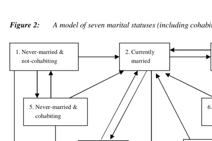
In this article, we employ a model that extends the four classical marital statuses to seven marital statuses that include cohabitation and combinations of cohabitation with other states (see Figure 2) (note 3).
1. Never-married & not-cohabiting 2. Married
3. Widowed & not-cohabiting 4. Divorced & not cohabiting 5. Never-married & cohabiting 6. Widowed & cohabiting 7. Divorced & cohabiting.
If cohabitation is negligible (or data concerning cohabitation are not available) in the study population, one may simply employ the classical four marital-status model; the procedures proposed in this article are still applicable when the transition rates relating to cohabitation are zero.
2. Computing Age-Specific Rates of Marriage/Union Formation and
Dissolution that are Consistent with the Projected Propensities in the
One-Sex Life Course Simulation Model
Figure 1: A model of four marital statuses
Figure 2: A model of seven marital statuses (including cohabitation)
1. Never married 2. Currently married
3. Widowed
4. Divorced
Death
1. Never-married & not-cohabiting
2. Currently married
3. Widowed & not-cohabiting
5. Never-married & cohabiting
6.Widowed & cohabiting
4. Divorced & not-cohabiting
7. Divorced & cohabiting
Changes in the propensity of one marital/cohabiting status transition affect the at-risk population and the number of events of other marital/cohabiting status transitions. For example, changes in the propensities of first marriage and remarriage cause changes in the at-risk population and the number of events of divorce. Changes in the propensity of divorce affect the at-risk population and the number of events of remarriage. The joint dependency between the number of events and the size of the at-risk population is the reason why one cannot achieve a projected x% change in the propensity of specified marital/cohabiting status changes simply by inflating or deflating the corresponding age-specific transition rates by x% (see Appendix A for a numerical illustration). Thus, we propose an iterative procedure to solve the problem.
The inputs and outputs of the iterative procedure for the model of seven marital statuses in Figure 2 are as follows:
Inputs:
A(i, j, s, t), the known (projected or assumed) sex-specific propensity of transition from marital/cohabiting status i to status j in life table cohort t, where the life table cohort t could be a period hypothetical cohort or a real cohort (note 5), and s = 1, 2 refers to females and males, respectively.
)
,
(
x
s
m
ijs , the known (or assumed) sex-age-specific standard (or initial) scheduleof rates of transition from marital/cohabiting status i to status j between ages x and x + 1, where i, j = 1, 2, 3, …, 7 (or 1, …, 4 if cohabitation is neglected).
Outputs:
mij(x, s, t), the sex-age-specific rate of transition from marital/cohabiting status i to
status j (i
≠
j) between ages x and x + 1 in the life table cohort t; the set of age-specifictransition rates, mij(x, s, t), is computed to yield A(i, j, s, t) as the resulting propensity. In general, the input and output variables are related as follows:
)
,
,
,
(
)
,
,
(
)
,
,
(
)
,
,
(
)
,
,
(
1t
s
j
i
A
t
s
x
m
t
s
x
L
t
s
x
m
t
s
x
L
ki k C k x x ij i=
∑
∑
∑
= = = ω α ω α, k ≠ i; i ≠ 1 (1)
where α is the lowest age at marriage and ω is the highest age considered in the life table model (e.g., 85); C is the number of marital/cohabiting statuses
distinguished; and Li(x, s, t) is the number of person-years lived in marital/cohabiting
Special considerations apply for i = 1. By convention, the life table cohort t
consists of 100,000 persons, all of whom enter the life course model at age α in
marital/cohabiting status 1 (never married and not cohabiting). It follows that:
)
,
,
2
,
1
(
000
,
100
)
,
,
(
)
,
,
(
12 1t
s
A
t
s
x
m
t
s
x
L
x=
∑
ω=α (2))
,
,
5
,
1
(
000
,
100
)
,
,
(
)
,
,
(
15 1t
s
A
t
s
x
m
t
s
x
L
x=
∑
ω=α. (3)
The propensities A(i, j, s, t) defined in formula (1) (k ≠ i; i ≠ 1) are lifetime
probabilities of transition from status i to j; A(1, 2, s, t) in formula (2) is the lifetime probability of experiencing first marriage. A(1, 5, s, t) in formula (3) is the average number of cohabitation unions before first marriage per person (note 6).
We now consider how one can compute sets of sex-age-specific transition rates,
mij(x, s, t), that are consistent with the known (projected or assumed) A(i, j, s, t) and the
known sex-age-specific standard schedule of transition rates,
m
ijs(
x
,
s
)
.Employing the matrix formula well established in the literature (see, e.g.,
Willekens, 1982; Schoen, 1988; Preston et al., 2001), we first use
m
ijs(
x
,
s
)
to estimate( , )
s ij
P x s
, the sex-age-specific probability of transition from marital/cohabiting status iat age x to marital/cohabiting status j at age x + 1 implied by the standard schedules.
Next, based on
P x s
ijs( , )
, we construct a multistate life table to get the sex-specificpropensities of marriage/union formation and dissolution implied by the standard schedules (As(i, j, s)).
We then use
(
,
)
)
,
,
(
)
,
,
,
(
)
,
,
(
1s
x
m
s
j
i
A
t
s
j
i
A
t
s
x
m
ij=
s ijs as the first approximation ofmij(x, s, t). We use the adjusted
(
,
,
)
1
t
s
x
m
ij to estimate(
,
,
)
1
t
s
x
P
ij ; we use)
,
,
(
1t
s
x
P
ij to construct a new multistate life table to get a new set of approximationsWe then use
(
,
,
)
)
,
,
,
(
)
,
,
,
(
)
,
,
(
1 12
t
s
x
m
t
s
j
i
A
t
s
j
i
A
t
s
x
m
ij=
ij as the secondapproximation of mij(x, s, t). We use the adjusted
(
,
,
)
2
t
s
x
m
ij to estimate)
,
,
(
2t
s
x
P
ij , we useP
ij2(
x
,
s
,
t
)
to construct a second multistate life table to get asecond set of approximations A2(i, j, s, t), which are not be equal to, but are closer to,
A(i, j, s, t) than are A1(i, j, s, t).
We continue this iterative process n times until all of the An(i, j, s, t) are almost
exactly equal to A(i, j, s, t). Generally, the convergence is sufficiently accurate when the absolute value of the largest relative discrepancy is less than 0.001, i.e.,
001
.
0
)
,
,
,
(
)
,
,
,
(
)
,
,
,
(
<
−
t
s
j
i
A
t
s
j
i
A
t
s
j
i
A
nfor all combinations of i, j, s, and t.
Using the above procedure, we conducted illustrative numerical applications of the four and seven marital/cohabiting status models using the U.S. 1990-1996 observed age-specific rates of marriage/union formation and dissolution as the standard schedules, based on the pooled data from four U.S. national surveys (note 7) (Zeng, Yang, Wang, and Morgan, 2002). We found that convergence of the iterative procedure
can be achieved and the goal of estimating sets of age-specific transition rates, mij(x, s,
t), that are consistent with the projected A(i, j, s, t) can be achieved. The number of
iterations required depends on the number of marital/cohabiting statuses distinguished in the model, the magnitude of the changes in the propensities, and the convergence criterion employed (e.g., the largest relative discrepancy). The illustrative applications are presented in Appendix A (note 8).
life table model that includes both nuclear and three-generation family households, and applied the extended model to Chinese data from 1950-1970 and 1981.
The family status life table models developed by Bongaarts (1987) and Zeng (1986; 1988; 1991) are female-dominant, one-sex life table models. Their applications assume that the age-specific demographic rates either remain constant at the values observed in a particular period in the past or vary according to the values observed for some real cohort; thus, it is not necessary to estimate time-varying age-specific rates for use in future years.
Using the procedure presented above, one can compute the time-varying age-specific rates to construct different one-sex family status life tables or other kinds of life course simulations for future years or cohorts using sex-age-specific standard schedules observed in the recent past and the projected or assumed propensities of marriage/union formation and dissolution in future years or for future cohorts. This can be done through macro or micro simulation approaches. Such exercises could clarify the implications of demographic changes on the life course in the one-sex dominant model.
For example, following a hypothetical cohort approach, one could simulate the impact on the expected number of years that women live in divorced status during the whole life course under the assumptions that female divorce propensity increases by 20%, remarriage propensity decreases by 15%, and first marriage propensity remain unchanged.
The procedure presented above can be regarded as an extension of the one-sex model for simulating the life course of a hypothetical (or real) cohort; however, it should not be used for projection purposes because it does not ensure the consistency across sexes required in the two-sex model for family household projections in monogamous societies. Specifically, in any given projection period, the total numbers of newly married (or cohabiting) men and women must be equal. Similar requirements must be formulated for the total numbers of divorces (or union dissolutions), numbers of new widows compared to married men who die, and vice versa. The adjustment procedure presented above does not ensure that the computed age-specific rates and the projected sex-specific propensities are consistent with the two-sex constraints on the future years’ sex-age-marital/cohabiting status distributions.
3. Computing Time-Varying Sex-Age-Specific Rates of
Marriage/Union Formation and Dissolution that are Consistent with
the Two-Sex Constraints and Projected Summary Measures in the
Family Household Projection Model
As discussed above, the time-varying sex-age-specific rates of marriage/union formation and dissolution must be estimated in a manner that ensures consistency between the sexes in the two-sex model of family household projections for monogamous societies. The procedures presented in this section are designed to ensure such consistency.
The estimated time-varying sex-age-specific rates must also be consistent with the independently projected summary measures of marriage/union formation and dissolution in future years. In specifying the summary measures of marriage/union formation and dissolution for family household projections, the following considerations will be important:
Whether the summary measures are appropriate for measuring the overall level and for ensuring the two-sex consistency;
Whether the summary measures are demographically interpretable, measurable, and predictable, and are easily understood by the public and by policy makers;
Whether the summary measures are sufficiently few in number for the model and applications to be manageable.
3.1 Two alternative groups of summary measures of marriage/union formation and dissolution
3.1.1 General rates of marriage/union formation and dissolution
The general rate of marriage/union formation and dissolution in projection year t is defined as the total number of events that would occur if the sex-age-specific rates of occurrence of the events in year t were applied to the most recent census-counted sex-age-marital/cohabiting-status distribution divided by the census-counted total number of males and females who were at risk of experiencing the events. Following the language used in Preston et al. (2001: 24), the general rate in projection year t is the general rate that would be estimated in year t if the population in year t retained its sex-age-specific rates but had the sex-age-marital/cohabiting-status distribution of the most recent census year (note 9).
We now provide formal definitions for the general rates employed in the model.
Let Ni(x, s, T0) denote the known number of persons of age x, marital/cohabiting
status i and sex s counted in the most recent census in year T0 (i.e., the starting
population of our family household projection) (note 10).
Let mij(x, s, t) be the sex-age-specific rates of transition from marital/cohabiting
status i to status j in year t (
i
≠
j
). The mij(x, s, t) are initially unknown; they arecomputed as outputs of the procedure.
Let GM(t) denote the projected general rate of marriages including first marriage and remarriage for males and females combined. It follows that:
GM(t) =
0 2
1,2
0 1,2
( , ,
)
( , , )
( , ,
)
i i
x s i
i
x s i
N x s T m
x s t
N x s T
β
α β
α = =
= =
∑ ∑ ∑
∑ ∑ ∑
, i = 1, 3, 4, 5, 6, 7 (4)where α is the lowest age at marriage and β is the upper bound of the age range in
which the general rate of marriage/union formation and dissolution is defined.
GD(t) =
2 0 24
1,2
2 0
1,2
( , ,
)
( , , )
( , ,
)
x s
x s
N x s T m
x s t
N x s T
β
α β
α = =
= =
∑ ∑
∑ ∑
. (5)Let GC(t) denote the projected general rate of cohabiting of never-married and ever-married males and females combined. It follows that:
GC(t) = 1 0 15 3 0 36 4 0 47
1,2
1 0 3 0 4 0 1,2
[ ( , , ) ( , , ) ( , , ) ( , , ) ( , , ) ( , , )]
[ ( , , ) ( , , ) ( , , )] x s
x s
N x s T m x s t N x s T m x s t N x s T m x s t
N x s T N x s T N x s T
β α
β α
= =
= =
+ +
+ +
∑ ∑
∑ ∑
. (6)
Let GCS(t) denote the projected general union dissolution rate for males and females combined. It follows that:
GCS(t)= 5 0 51 6 0 63 7 0 74
1,2
5 0 6 0 7 0
1,2
[ ( , , ) ( , , ) ( , , ) ( , , ) ( , , ) ( , , )]
[ ( , , ) ( , , ) ( , , )] x s
x s
N x s T m x s t N x s T m x s t N x s T m x s t
N x s T N x s T N x s T
β α
β α
= =
= =
+ +
+ +
∑ ∑
∑ ∑
. (7)
3.1.2 Overall propensities of marriage/union formation and dissolution in the context of the period life table
Let Li(x, t) denote the life table number of person-years lived in marital/cohabiting
status i between ages x and x + 1 in the combined male and female period life table in
year t; Li(x, t) is a derived variable computed through life table construction based on
mij(x, t).
Let PM1(t) denote the projected propensity of first marriage (i.e., the probability of experiencing first marriage) during the life course if the sex-age-specific rates of marriage/union formation and dissolution in year t are applied to a hypothetical cohort of males and females combined.
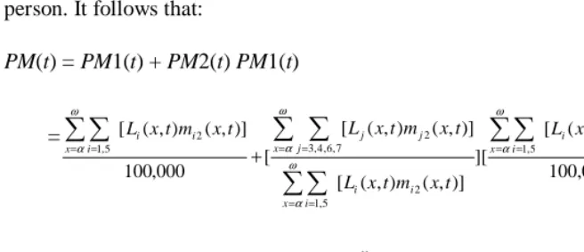
propensity of marriage in the context of the period life table; PM(t) is actually the average number of marriages (including first marriage and remarriages) per average person. It follows that:
PM(t) = PM1(t) + PM2(t) PM1(t) (8a)
= ] 000 , 100 )] , ( ) , ( [ ][ )] , ( ) , ( [ )] , ( ) , ( [ [ 000 , 100 )] , ( ) , ( [ 2 5 , 1 2 5 , 1 2 7 , 6 , 4 , 3 2 5 , 1
∑∑
∑∑
∑ ∑
∑∑
= = = = = = = = + ω α ω α ω α ω α x i i i x i i i x j j j x i i i t x m t x L t x m t x L t x m t x L t x m t xL (8b)
=
000
,
100
)]
,
(
)
,
(
[
000
,
100
)]
,
(
)
,
(
[
2 7 , 6 , 4 , 3 2 5 ,1
∑ ∑
∑ ∑
= = = =+
ω α ω α x j j j x i i it
x
m
t
x
L
t
x
m
t
x
L
(8c)where α is the lowest age at marriage and ω is the highest age considered in the life table.
Let PD(t) denote the projected overall propensity of divorce of an average person during the life course if the sex-age-specific rates of marriage/union formation and dissolution in year t are applied to a hypothetical cohort of males and females combined. It follows that:
PD(t) = 2 24 2 2
( , )
( , )
[ ( , )
( , )]
x i i x iL x t m
x t
L x t m
x t
ω α ω α = = ≠
∑
∑∑
. (9)Let PC1(t) denote the average number of cohabitation unions before first marriage per person during the life course if the sex-age-specific rates of marriage/union formation and dissolution in year t are applied to a hypothetical cohort of males and females combined.
We combine PC1(t) and PC2(t) into one index, PC(t), the projected overall propensity of cohabitation in the context of the period life table; PC(t) is actually the average number of cohabitation unions (both before first marriage and after first marriage dissolution) per average person. It follows that:
PC(t)= PC1(t) +PC2(t) PM1(t) (10a)
= ] 000 , 100 )] , ( ) , ( [ ][ )] , ( ) , ( [ )] , ( ) , ( ) , ( ) , ( [ [ 000 , 100 )] , ( ) , (
[ 1 12
12 1 47 4 36 3 15 1
∑
∑
∑
∑
= = = = + + ω α ω α ω α ω α x x x x t x m t x L t x m t x L t x m t x L t x m t x L t x m t xL (10b)
=
000
,
100
)]
,
(
)
,
(
)
,
(
)
,
(
[
000
,
100
]
)
,
(
)
,
(
[
1 15∑
3 36 4 47∑
= =∂+
+
ω ω α x xt
x
m
t
x
L
t
x
m
t
x
L
t
x
m
t
x
L
. (10c)Let PCS(t) denote the overall propensity of cohabitation union dissolution of an average person who has ever cohabitated during the life course if the sex-age-specific rates of marriage/union formation and dissolution in year t are applied to a hypothetical cohort of males and females combined. It follows that:
PCS(t) =
)]
,
(
)
,
(
)
,
(
)
,
(
)
,
(
)
,
(
[
)]
,
(
)
,
(
)
,
(
)
,
(
)
,
(
)
,
(
[
47 4 36 3 15 1 74 7 63 6 51 5t
x
m
t
x
L
t
x
m
t
x
L
t
x
m
t
x
L
t
x
m
t
x
L
t
x
m
t
x
L
t
x
m
t
x
L
x x+
+
+
+
∑
∑
= = ω α ω α . (11)3.1.3 Rationale, assumptions, and implications of the summary measures
We now discuss several important issues relating to the rationale, assumptions, and implications of the two alternative groups of summary measures presented above.
(1) The summary measures are defined for males and females combined.
consistent with the two-sex constraints. This is because the two-sex constraints also depend on the unknown (to-be-projected) sex-age-marital/cohabiting- status distributions in future years.
Although we employ the summary measures of marriage/union formation and dissolution for males and females combined (note 11), we compute and use the sex-age-specific rates of marriage/union formation and dissolution (see Section 3.2) to derive changes in the marital/cohabiting status of individuals in the population. This strategy (1) reproduces the summary measures for the two sexes combined, (2) estimates the sex-age-specific rates in the detailed calculations, and (3) satisfies the two-sex constraints. Thus, this strategy adequately models the overall levels and gender differentials of marriage/union formation and dissolution.
(2) Standardization by age and marital/cohabiting status is important.
The summary measures in different projection years must be standardized by age and marital/cohabiting-status in order to eliminate possible biases in measuring changes in the levels of marriage/union formation and dissolution due to cross-period changes in the age structure and marital/cohabiting statuses of the population. For example, the not–age-standardized general marriage (or divorce) rate – defined as the total number of marriages (or divorces) divided by the total number of not-married (or currently married) persons in year t – would decrease/increase purely due to the structural growth/decline of the numbers of elderly even if the level of marriage (or divorce) at each age does not change. This is because the rates of marriage (or divorce) of the elderly are substantially lower than those of younger people.
We define the standardized general rates of marriage/union formation and dissolution using the age and marital/union status distributions in the starting year of projection (i.e., the most recent census observations) as the “standard”. We follow the multistate period life table approach in defining the overall propensities of
marriage/union formation and dissolution based on the sex-age-specific rates, mij(x, s,
t), which are standardized for age and marital/cohabiting status structures and take into account both the occurrences of and exposures to the relevant events (note 12).
different non-marital statuses. Thus, we define the overall summary measures of marriage/union formation (GM(t), GC(t), PM1(t), PM2(t), PC1(t), and PC2(t)) to include relevant events with different marital statuses before the onset of marriage or cohabitation. This implies that the changes in the overall intensities of various marriages and cohabitations are assumed to be proportional to the changes in the overall summary measures. This assumption is generally reasonable since different kinds of marriages/cohabitations are all related to general social attitudes towards marriage and cohabitation.
An analyst who is not satisfied with such an assumption could simply inflate or deflate the rates within the standard schedules (estimated from survey data) of sex-age-specific rates of marriage/cohabitation of never-married, widowed, and divorced persons differently according to some alternative set of assumptions, to reflect the speculated differentials in future years, while the overall summary measures would continue to reflect the general levels of marriage/union formation.
Combining the detailed sex–age–marital/cohabiting-status–specific rates with the overall summary measures of marriage/union formation is a reasonable approach for modeling differentials in marriage/cohabitation among different types of unmarried persons, while meeting the two-sex constraints. Indeed, as described in Section 3.2, the sex-age-specific rates of marriage/union formation are computed separately for persons with different marital statuses before the onset of marriage and cohabitation, respectively. Furthermore, one can easily calculate the implied values of the more detailed sex-specific summary measures of first marriage, remarriage, or cohabitation of never-married and ever-married persons in year t once the sex-age-specific rates of
marriage/union formation and dissolution in year t (i.e., the mij(x, s, t)) have been
computed.
(4) Practical considerations limit the age range used in computing the summary measures.
bound; we also use the estimated standard schedules of sex-age-specific rates at ages above the upper bound (e.g., estimated by averaging over longer time periods or by using fitted parametric models) to determine the age pattern of marriage/union formation and dissolution at older ages.
3.2 Procedure for computing sex-age-specific rates which are consistent with the two-sex constraints and the projected summary measures
The inputs and outputs of the iterative procedure for the two-sex model of seven marital statuses in Figure 2, specified to ensure consistency with the two-sex constraints and the projected summary measures, are as follows:
Inputs:
The known (projected or assumed) general rates of marriage/union formation and dissolution in each projection year t (i.e., GM(t), GD(t), GC(t), and GCS(t)); or the known (projected or assumed) propensities of marriage/union formation and dissolution in each projection year t (i.e., PM1(t), PM2(t), PD(t), PC1(t), PC2(t), and PCS(t)).
)
,
(
x
s
m
ijs , the known sex-age-specific standard schedule of rates of transitionfrom marital/cohabiting status i to status j between ages x and x + 1.
Outputs:
mij(x, s, t), the sex-age-specific rate of transition from marital/cohabiting status i to
status j (i
≠
j) between ages x and x + 1 in projection year t; the set of sex-age-specifictransition rates is computed to be consistent with the two-sex constraints and the projected summary measures.
The iterative procedure consists of repeated applications of two basic steps.
Step 1. Adjustments to satisfy the two-sex constraints, following the harmonic mean approach
Step 2. Adjustments to achieve consistency with the summary measures of marriage/union formation and dissolution in year t
To compute sets of unknown mij(x, s, t) that are consistent with the general rates
GM(t), GD(t), GC(t), and GCS(t), we perform a second set of adjustments based on the
adjusted sex-age-specific transition rates, m'ij(x, s, t), estimated in Step 1, which were
constructed to meet the two-sex constraints (see Appendix B for more details). We use the same adjustment factors for adjusting male and female rates to help maintaining the two-sex consistency achieved in Step 1. These adjustments are implemented as follows:
)
,
,
(
'
)
(
'
)
(
)
,
,
(
'
'
2m
2x
s
t
t
GM
t
GM
t
s
x
m
i=
i , i = 1, 3, 4, 5, 6, 7 (12))
,
,
(
'
)
(
'
)
(
)
,
,
(
'
'
24m
24x
s
t
t
GD
t
GD
t
s
x
m
=
(13))
,
,
(
'
)
(
'
)
(
)
,
,
(
'
'
15m
15x
s
t
t
GC
t
GC
t
s
x
m
=
(14))
,
,
(
'
)
(
'
)
(
)
,
,
(
'
'
36m
36x
s
t
t
GC
t
GC
t
s
x
m
=
(15))
,
,
(
'
)
(
'
)
(
)
,
,
(
'
'
47m
47x
s
t
t
GC
t
GC
t
s
x
m
=
(16))
,
,
(
'
)
(
'
)
(
)
,
,
(
'
'
51m
51x
s
t
t
GCS
t
GCS
t
s
x
m
=
(17))
,
,
(
'
)
(
'
)
(
)
,
,
(
'
'
63m
63x
s
t
t
GCS
t
GCS
t
s
x
m
=
(18))
,
,
(
'
)
(
'
)
(
)
,
,
(
'
'
74m
74x
s
t
t
GCS
t
GCS
t
s
x
m
=
, (19)where GM(t), GD(t), GC(t), and GCS(t) are the projected (or assumed) general rates;
and GM'(t), GD'(t), GC'(t), and GCS'(t) are derived by substituting m'ij(x, s, t) in
Additional Considerations
The adjustments described in Step 1 are based on
N
'
i(
x
,
s
,
t
)
, the mid-yearpopulations, classified by age, sex, and marital/cohabiting status (see Appendix B).
)
,
,
(
'
x
s
t
N
i is the average of the populations at the beginning (Ni(x, s, t)) and the end(Ni(x + 1, s, t + 1)) of year t. Each
N
'
i(
x
,
s
,
t
)
only approximatesN x s t
i( , , )
, sincethe calculation of
N
'
i(
x
,
s
,
t
)
is based on the approximation of the sex-age-specificrates (m'ij(x, s, t)).
Moreover, although we use the same adjustment factors for males and females in Step 2, the adjusted rates in Step 2 will not exactly satisfy the two-sex constraints
because the
N
'
i(
x
,
s
,
t
)
are not the final estimates.Therefore, we need to use the
m
'
'
ij(
x
,
s
,
t
)
estimated in Step 2 to computeanother iteration of Step 1, with the new population counts, denoted by N''i(x + 1, s, t +
1) and
N
''
i(
x
,
s
,
t
)
, computed using formulas (B-1) and (B-2) in Appendix B.We next use
N
'
'
i(
x
,
s
,
t
)
andm
"
ij(
x
,
s
,
t
)
to replaceN
'
i(
x
,
s
,
t
)
and mij(x,s,t–1) in formulas (B-3) – (B-19) in Appendix B, repeating the adjustment procedure described therein, to obtain new estimates of the sex-age-specific rates, denoted by m'''ij(x, s, t), which satisfy the two-sex constraints.We then use the new estimates of m'''ij(x, s, t) to compute another iteration of Step
2, obtaining new estimates of the general rates of marriage/union formation and dissolution, denoted by GM''(t), GD''(t), GC''(t), and GCS''(t).
If the absolute values of the relative differences between the new estimates of the general rates and the corresponding projected general rates are all less than the selected convergence criterion (e.g., 0.01 or 0.001), then we have obtained a solution for computing the sex-age-specific rates in year t that satisfies the two-sex constraints and reproduces the projected summary measures. Otherwise, we need further iterations of the adjustment procedures in Steps 1 and 2, as described above, until the convergence criterion is met.
Illustrative Applications
To develop numerical examples, we used the procedure described above in Steps 1 and 2 with the general rates and the overall propensities as summary measures, respectively, to compute the time-varying sex-age-specific rates of marriage/union formation and dissolution over the projection interval from 2000 to 2050. The standard schedules were based on the estimates of the U.S. sex-age-specific rates of marriage/union formation and dissolution in 1990-1996 (Zeng et al., 2002). The sex– age–marital/cohabiting-status distributions at the starting year of the projection were derived from the U.S. 2000 census micro sample data file. We estimated models with seven marital/cohabiting statuses including cohabitation (Figure 2) for four race groups. The required number of repetitions of Steps 1 and 2 using general rates as summary measures was between 2 and 4, as indicated in Table 1.
Table 1: Number of repetitions of Steps 1 and 2 (assuming that GM(t) decreases by 4%, GD(t) increases by 5%, GC(t) increases by 8%, and GCS(t) increases by 6%)
Criterion (relative difference): 0.01 Criterion (relative difference): 0.001
All races combined Four race groups All races combined Four race groups
2 3 3 4
The required number of repetitions of Steps 1 and 2 using overall propensities as summary measures was between 2 and 5, as indicated in Table 2.
Table 2: Number of repetitions of Steps 1 and 2 (assuming that PM(t) decreases by 4%, PD(t) increases by 5%, PC(t) increases by 8%, and PCS(t) increases by 6%)
Criterion (relative difference): 0.01 Criterion (relative difference): 0.001
All races combined Four race groups All races combined Four race groups
The results in Tables 1 and 2 demonstrate that the iterative procedures expressed in Steps 1 and 2 are valid for practical applications. In both applications, the required number of iterations was much smaller than that for the one-sex life course simulation model procedure, which involved much more detailed propensities of marriage/union status transitions (presented in Section 2 with illustrative numerical example in Appendix A).
Based on the final estimates of mij(x, s, t) in year t, one can also construct
multistate life tables for males and females separately and compute the detailed sex-specific period life table propensities of transitions from marital/cohabiting status i to
status j, PPij(s, t), in year t. The PPij(s, t), which reflect gender differentials in the
intensities of transitions among various marital/cohabiting statuses are consistent with the two-sex constraints and the projected summary measures in the projection years.
4. Concluding Remarks
Family household projections/simulations and other relevant projections/simulations (e.g., actuarial and welfare forecasting) often require computation of time-varying sex-age-specific rates of marriage/union formation and dissolution which match the projected (or assumed) summary measures of marriage/union formation and dissolution in future years. In the applications of family household projections/simulations for monogamous populations, consistency across the sexes must also be ensured. The computation cannot be done by simply inflating or deflating each set of age-specific rates independently as typically done in computing fertility rates in classical population projections. This is because changes in the propensity of one status transition affect the at-risk population and the number of events of other status transitions and because the two-sex constraints must be met.
This article presents a procedure for computing sex-age-specific rates which ensure that the projected propensities of marriage/union formation and dissolution are achieved consistently in the one-sex life course simulation model. Another more practically useful procedure for computing sex-age-specific rates which are consistent with the two-sex constraints and which reproduces the projected summary measures of marriage/union formation and dissolution in future years in the two-sex family household projection model was also proposed.
We define, discuss, and employ two alternative groups of summary measures in the two-sex family household projection model: (1) general rates – GM(t), GD(t),
GC(t), and GCS(t); and (2) overall propensities – PM1(t), PM2(t), PD(t), PC1(t), PC2(t), and PCS(t). Both groups of summary measures are appropriate for measuring
the two-sex constraints; the summary measures are all demographically interpretable, measurable, and predictable; and each group has only four or six summary parameters to be projected, which makes the model and its applications manageable.
Compared to the general rates, the overall propensities are relatively easier for the public and policy makers to understand. For example, a report that the divorce level in year t implies that 35 percent of marriages would eventually end in divorce is more informative to the public and policy makers than a report of the general rate of divorce. This is useful in policy analysis.
On the other hand, time series of GM(t) and GD(t) are likely to be available from vital statistics at both national and provincial/state levels. Trends of period average
GC(t) and GCS(t) (e.g., five-year averages) can be estimated from retrospective surveys
that collect cohabitation information. Thus, projecting GM(t), GD(t), GC(t), and GCS(t) based on time series extrapolations would be relatively more feasible, which would facilitate forecasting for market analysis and business planning purposes.
Time series estimation of the multistate life table propensities PM1(t), PM2(t),
PD(t), PC1(t), PC2(t), and PCS(t), however, needs intensive historical time series data
on sex-age-specific rates, including occurrences of and exposures to marriage/union formation and dissolution, which may be difficult to obtain or not available at all, especially at provincial/state levels. Thus, time series extrapolation of the overall propensities PM1(t), PM2(t), PD(t), PC1(t), PC2(t), and PCS(t) may not be possible for household forecasting for business/planning purposes at the provincial/state level. The use of the overall propensities is more informative in policy analyses/scenarios at the national level, and such analyses can be done without the time series extrapolation.
The general rates GM(t), GD(t), GC(t), and GCS(t), which are more likely to be available based on time series extrapolation, are recommended for short-term family household forecasts for market analysis and business planning purposes.
If the general rates are chosen, one can also compute the implied corresponding period life table propensities of marriage/union formation and dissolution in the starting and future projection years (e.g., A(i, j, s, t); see formulas (1), (2), and (3)), so that these implied, more informative summary measures may be reported.
projections also need to reasonably compute the time-varying age-parity-specific rates of marital and non-marital fertility and other time-varying sex-age-specific rates such as mortality, migration, and leaving the parental home, based on the projected summary measures and the standard schedules; these tasks are beyond the scope of this article, but certainly deserve attention.
5. Acknowledgements
An earlier version of this paper was prepared for the NIA sponsored workshop on "Future Seniors and Their Kin" in honor of Professor E.A. Hammel’s retirement with
outstanding career contributions to demography, April 5-7, 2002, Berkeley, CA.
Notes
1. When first marriage and/or fertility are delayed or advancing, for example, one
may shift the age-specific standard schedules of first marriage and/or fertility to the right or left by the amount of increase or decrease in the mean age at first marriage and/or fertility, while the shape of the schedules remains unchanged. One may also assume that first marriage and/or fertility would be delayed or advanced while the curves become more spread or more concentrated through parametric modeling (Zeng et al., 2000).
Zeng, Yang, Wang, and Morgan (2002) recently estimated the U.S. race-sex-age-specific occurrence/exposure (o/e) rates of marriage/union formation and dissolution and the race–age–parity–marital-status–specific rates of fertility in the 1970s, 1980s, and 1990s. This work was based on pooled data from 10 waves of four major national surveys conducted from 1980 to 1996 (with a total sample size of 394,791 women and men). The estimates showed empirically that the basic shapes of the demographic schedules remained reasonably stable from the 1970s to the 1990s, while the timing was changing. We, thus, may reasonably assume that in normal circumstances the basic shapes of the standard schedules remain approximately stable, while the changes in timing are modeled through the changing mean age at marriage and fertility in the family household projection.
2. These “rates” are actually occurrence/exposure rates, but we use the word “rates”
for simplification.
3. We do not include “married & legally separated from legal spouse but cohabiting
with a partner” because of the unavailability of data on such cases and because we wish to simplify the model. “Legal separation” is combined with “Divorced” to simplify the model. One may consider grouping never-married & cohabiting, widowed & cohabiting, and divorced & cohabiting into one status of “cohabiting”, which leads to a simpler model that contains five statuses only. In a five-status model, however, the three kinds of cohabiting people with different legal marital statuses (never-married, widowed, and divorced) are not distinguishable and they are all mixed into “single” once their union is broken. Such a grouping of the never-married, widowed, and divorced into one “single” status is not appropriate because these three kinds of people are likely to behave differently.
4. The term “propensity of marriage/union formation and dissolution” in this article is
age-specific probabilities of marital status transitions, which are frequently used. Moreover, “propensity” is a broader concept which includes not only “probabilities of marital status transitions” in this article as used by Schoen (1988: 95), but also a few additional summary measures used in this article which are not probabilities, e.g., average number of cohabitation unions before first marriage per person (A(1, 5, s, t)), defined in Section 2, and average number of remarriages per ever-married person (PM2(t)), defined in Section 3.
5. Note that the index “t” in all variables in Section 2 refers to the period hypothetical
cohort life table or the real cohort in the one-sex life course simulation model. The index “t” in all variables in Section 3 refers to calendar year because we deal with two-sex family household projection models there.
6. One may consider an alternative definition of A(1, 5, s, t): “life-time probability of
transition from never-married to cohabitation”:
)
,
,
5
,
1
(
)
,
,
(
)
,
,
(
000
,
100
)
,
,
(
)
,
,
(
51 5
15 1
t
s
A
t
s
x
m
t
s
x
L
t
s
x
m
t
s
x
L
x
=
+
∑
= ω
α
.
This alternative definition implicitly assumes that the probability of entering the second and higher order unions before first marriage among those whose first union was broken (i.e.,
L
5(
x
,
s
,
t
)
m
51(
x
,
s
,
t
)
) is the same as the probability of entering the first union among those initial life table cohort members at the lowestage of marriage, α (i.e., 100,000). This assumption may not reasonable. Moreover,
our trial exercise using this alternative definition shows that it significantly increases the number of iterations (and thus computing time) needed for convergence (see Appendix A for more details about the convergence criteria).
7. The four national surveys were (a) 1980, 1985, 1990, and 1995 Current Population
Survey (CPS); (b) 1987-1988 and 1992-1994 National Survey on Family Households (NSFH); (c) 1982, 1988, and 1995 National Survey on Family Growth (NSFG); and (d) 1996 Survey on Income and Program Participation (SIPP). The pooled data set had a total sample size of 296,988 women and 97,803 men (Zeng, Yang, Wang, and Morgan, 2002).
8. We present summary results from the illustrative numerical applications verifying
standard schedules and estimated time-varying age-specific rates of marriage/union formation and dissolution due to space limitations.
9. “t" refers to future calendar years here, but it may also refer to calendar years in the
past. We may estimate the general rates of marriage/union formation and dissolution in the past by combining the same “standard” sex-age distribution of the population observed from the most recent census with the time-varying sex-age-specific rates in the past. Use of these general rates for past years will eliminate possible distortions caused by temporal changes in the age structure of the population. If time-varying sex-age-specific rates in the past are not available, one may estimate the general rates in the past by dividing the total number of events in the past by the total number of persons at risk of experiencing the events in the past. In such cases, the researcher will need to detect and adjust for any bias caused by temporal changes in the population age structure using other demographic methods, such as the indirect estimation method.
10. If the population in the household projection model is stratified by race or by
rural-urban sectors, a similar stratification can be imposed on the “standard” sex–age–
marital-status distribution, Ni(x, s, T0), for all races combined, or for rural-urban
sectors combined, as counted in the most recent census. This allows one to standardize the age distributions not only across time, but also across race groups or rural-urban sectors, to eliminate possible distortions in measuring levels of marriage/union formation and dissolution due to changes in age structures in different years and between race groups or rural-urban sectors.
11. In monogamous societies in a given year, the number of currently married (or
cohabiting) males is equal to the number of currently married (or cohabiting) females; the total numbers of newly divorced (or union broken) men and women are also equal. Thus, the overall probabilities of divorce (or union break) of men and women should be equal and defining summary measures of divorce (or union break) for men and women combined is reasonable. In contrast, although the numbers of newly marrying (or newly cohabiting) men and women are equal, the overall probabilities of marriage/cohabitation of men and women are not necessarily the same because males and females who are eligible (or at risk) to newly marry (or newly cohabit) may not be equal. Thus, the summary measures of marriage/cohabitation for men and women combined indicate the average intensity of marriage/union formation across the sexes.
12. We cannot use the total rates of the non-repeatable events (such as order-specific
they may be seriously distorted due to changes in tempo (see, e.g., Ryder 1964; 1980; 1983; Keilman, 1995; Van Imhoff and Keilman, 1995; Bongaarts and Feeney, 1998; Kim and Schoen, 2000; Kohler and Philipov, 2001; Van Imhoff and Keilman, 2000; Zeng and Land, 2001; 2002).
13. Once reliable age-sex-specific standard schedules for a country have been
estimated (and updated every few years, depending on data availability) by a researcher, however, others could simply employ these standard schedules as “model standard schedules” for household forecasting at the country or provincial/state level. This is because, while the projected demographic summary measures are crucial, the forecasting results are not substantially sensitive to the age-specific model standard schedules as long as they reveal the general age pattern of the demographic process of the population; this statement has been corroborated by the sensitivity analysis reported in Zeng, Land, Wang, and Gu (2004).
14. The following case of first marriage rates/propensity serves as an example; the
propensity of first marriage in the life course is defined in formula (2) in the text.
Let α = 15, m12(15, s, t) = 0.1, m12(16, s, t) = 0.1,
L1(15, s, t) = [100,000 + (100,000 – 100,000 * 0.1)]/2 = 95,000,
L1(16, s, t) = [90,000 + (90,000 – 90,000 * 0.1)] /2= 85,500.
After each m12(x, s, t) is inflated by 8%, m'12(15, s, t) = 0.108, m'12(16, s, t) = 0.108,
L'1(15, s, t) = [100,000 + (100,000 – 100,000 * 0.108)]/2 = 94,600,
L'1(16, s, t) = [89,200 + (89,200 – 89,200 * 0.108)] /2= 84,383.
The above numerical calculation clearly shows that after each m12(x, s, t) is inflated
by 8%, L'1(x, s, t) is reduced at every age compared to L1(x, s, t), which corresponds
to keeping m12(x, s, t) unchanged. Thus, the new A'(1, 2, s, t) (computed by formula
References
Bongaarts, J. 1987. “The projection of family composition over the life course with family status life tables.” In: Bongaarts, J., T. Burch and K.W. Wachter (eds.)
Family Demography: Methods and Applications. Oxford: Clarendon Press.
Bongaarts, J. and G. Feeney. 1998. “On the Quantum and Tempo of Fertility.”
Population and Development Review 24 (2): 271-291.
George, M.V. 1999. “On the Use and Users of Demographic Projections in Canada” Working Paper No. 15, Conference of European Statisticians, Joint ECE-EUROSTAT work session on Demographic Projections (Perugia, Italy, 3-7 May 1999).
Gill, R.D. and N. Keilman 1990. “On the estimation of multidimensional demographic models with population registration data” Mathematical Population Studies 2, 119-143.
Keilman, N. 1985. “Nuptiality Models and the Two-Sex Problem in National Population Forecasts.” European Journal of Population Vol. 1(2/3), pp. 207-235.
Keilman, N. 2003. “The threat of small households.” Nature, Vol. 421: 489-490.
Keilman, N. 1994. “Translation Formulae for Non-Repeatable Events.” Population
Studies 48: 341-357.
Keilman, N. and E.V. Imhoff. 1995. “Cohort quantum as a function of time-dependent period quantum for non-repeatable events.” Population Studies 49: 347-352.
Keyfitz, N. 1972. “On Future Population.” Journal of American Statistical Association, 67: 347 - 363.
Kim, Y.J. and R. Schoen. 2000. "Changes in Timing and the Measurement of Fertility."
Population and Development Review 26: 554-59.
Kohler, H.P. and M. Philipov. 2001. “Variance effects in the Bongaarts-Feeney formula”. Demography 38 (1): 1-16.