Classifier System Learning of Good Database Schema

(1)

University of New Orleans University of New Orleans

ScholarWorks@UNO

University of New Orleans Theses and

Dissertations Dissertations and Theses

8-7-2008

Classifier System Learning of Good Database Schema

Mitsuru Tanaka

University of New Orleans

Follow this and additional works at: https://scholarworks.uno.edu/td

Recommended Citation Recommended Citation

Tanaka, Mitsuru, "Classifier System Learning of Good Database Schema" (2008). University of New Orleans Theses and Dissertations. 859.

https://scholarworks.uno.edu/td/859

This Thesis is protected by copyright and/or related rights. It has been brought to you by ScholarWorks@UNO with permission from the rights-holder(s). You are free to use this Thesis in any way that is permitted by the copyright and related rights legislation that applies to your use. For other uses you need to obtain permission from the rights-holder(s) directly, unless additional rights are indicated by a Creative Commons license in the record and/or on the work itself.

(2)

Classifier System Learning of Good Database Schema

A Thesis

Submitted to the Graduate Faculty of the University of New Orleans in partial fulfillment of the requirements for the degree of

Master of Science in

The Department of Computer Science

By

Mitsuru Tanaka

B.E., Hiroshima Kokusai Gakuin University, Japan, 2001

(3)

(4)

Dedication

This thesis is dedicated to my parents Mr. Chiaki Tanaka and Mrs. Hisako Tanaka,

(5)

Acknowledgement

I would like to thank my thesis advisor Dr. Shengru Tu. Dr. Tu introduced me to a

research project, which required knowledge of database and artificial intelligence fields

and later motivated me to write a thesis on it. Artificial intelligence was a frontier field to

me. The fusion of the two fields presented many questions for me to explore in the

project. I thank Dr. Tu for answering to my questions and being supportive throughout

the completion of my thesis.

I would also like to thank Dr. Adlai DePano, and Dr. Golden Richard, III, for

becoming my thesis committee members.

I would also like to thank Dr. Lingyan Shu, who was the team leader in the

project, for helping me in the artificial intelligence studies.

I would also like to thank other faculty members and staffs for providing me with

(6)

List of Figures

Figure 1.1: Alternatives for CUSTOMER and TELEPHONE ...4

Figure 1.2: An E-R Diagram without CUSTOMER Entity Set...5

Figure 2.1: A Six-Bit Multiplexer Function ...14

Figure 3.1: A Mountain with a Single Peak...17

Figure 3.2: A Mountain with Multiple Peaks ...18

Figure 3.3: Noisy and Discontinuous Functions...19

Figure 3.4: Roulette Wheel for Reproduction...22

Figure 3.5: An Example Binary Representation of the Strings in a Knapsack Problem .31 Figure 3.6: A Learning Classifier System Interacting with its Environment ...35

Figure 4.1: The Input to the Classifier System ...41

Figure 4.2: System Tab with the Output...42

Figure 4.3: The Declarations of ClassType...43

Figure 4.4: The Declarations of PopType...44

Figure 4.5: An Iteration of the Classifier System ...45

Figure 4.6: The Class Diagram of Perform...46

Figure 4.7: The Class Diagram of AOC...47

Figure 4.8: The Class Diagram of GA...48

Figure 4.9: The Class Diagram of Reinforc...49

Figure 4.10: The Class Diagram of RewardCalculator...50

Figure 4.11: The Method matchclassifiers...51

Figure 4.12: Some Classifiers Matching to an Environmental Message ...52

Figure 4.13: The Method auction...53

Figure 4.14: The Method taxcollector...54

Figure 4.15: Relations and Mapping Cardinalities ...56

Figure 5.1: Well-Designed Input Schema...58

Figure 5.2: Mapping Cardinalities of the Well-Designed Input Schema...58

Figure 5.3: Initial Population Generated From the Well-Designed Input Schemas ...58

Figure 5.4: Top Five Classifiers of the Final Population in the Experiment with the Well-Designed Schemas ...59

Figure 5.5: Number of Classifiers with Strength Over 2 ...60

Figure 5.6: Number of Classifiers with Strength Over 10 ...60

Figure 5.7: Input in Which PROJ Is Modified...61

Figure 5.8: Initial Population Generated From the Badly Designed Input Schemas...61

(9)

List of Tables

Table 3.1: Example of Four Strings...21

Table 3.2: Four Strings with 0 Fitness Value ...24

Table 3.3: The Effect of Mutation ...25

Table 3.4: Weight and Profit of the Items for a Knapsack Problem...30

Table 3.5: String and Schema Processing by Genetic Algorithms for a Knapsack Problem...32

(10)

Abstract

This thesis presents an implementation of a learning classifier system which

learns good database schema. The system is implemented in Java using the NetBeans

development environment, which provides a good control for the GUI components. The

system contains four components: a user interface, a rule and message system, an

apportionment of credit system, and genetic algorithms. The input of the system is a set

of simple database schemas and the objective for the classifier system is to keep the good

database schemas which are represented by classifiers. The learning classifier system is

given some basic knowledge about database concepts or rules. The result showed that the

system could decrease the bad schemas and keep the good ones.

Keywords and Phrases: classifier system, machine learning, genetic algorithms, and

(11)

Chapter 1: Introduction

A classifier system is a machine learning system which uses genetic algorithms.

Genetic algorithms are based on the principle of Darwin’s survival of the fittest. They are

derived from a computational model of evolutionary genetics. They also have been

applied to search and optimization problems. Genetic algorithm based classifier systems

have been applied to a variety of learning tasks. In this thesis, the classifier system is

applied to learn good relational database schemas.1

1.1 Applying the Classifier System to the Learning of Good Database

Schema

Database design involves complex tasks. Databases are widely used in banking,

airlines, universities, or credit card transactions. Such databases are designed to manage

large bodies of information. To map the information to relational database, there are

many steps involved in the design. Database design usually involves the following phases

[1]: characterizing the data needs of the prospective database users, conceptual-design,

creating a specification of functional requirements, logical design, and physical design. In

these phases, there are many concepts, theories, or rules, which help the database

designers to produce good database schemas. These five phases involve complex tasks

when the information is large.

1

(12)

In the first phase to characterize the data needs of the prospective database users,

the database designer needs to interact extensively with domain experts and users to carry

out this task. The output of this phase is a specification of user requirements. If the client

is a bank, there may be a requirement that all the customers must be identified by their

customer identification values. In addition, there may be a requirement that a customer

must always be associated with a particular banker, who may act as a loan officer or

personal banker for that customer. Because of the first requirement, the database designer

must set up a constraint that the identification value given to the customer cannot be

assigned to other customers. The second requirement raises a question: what if the banker

associated with a customer quits? As the information gets complex, the requirements can

be large. These requirements or restrictions tend to complicate the designing of databases.

In the conceptual-design phase, the database designer translates the specification

of requirements to a conceptual schema of the database. The output is a schema that

provides a detailed overview of the enterprise. Usually, the entity-relationship model

(E-R model) [2] is used for this purpose. The output schema is described as an

entity-relationship diagram with the E-R model.

In the E-R model, a thing or object in the real world that is distinguishable from

all other objects is called an entity. For example, each person in an enterprise is an entity.

An entity is represented by a set of attributes, which are descriptive properties possessed

by each member of an entity set. For example, a person at a bank with an identification

number, a name, or a street may be the example attributes. An entity set is a set of entities

of the same type that share the same properties, or attributes. Therefore, the all customers

(13)

entities is defined as a relationship in the E-R model. For example, the relation between a

customer named Johnson and his associated banker named Smith can be described as a

relationship. A relationship set is a set of such relationships of the same type. The

relationships between customer and associated banker entity sets can be described as a

relationship set. Even though the E-R model captures such semantics among data and

depicts in an E-R diagram, there are some known issues.

Consider the entity set CUSTOMER with its attributes CUSTOMER_ID,

CUSTOMER_NAME, CUSTOMER_CITY, and CUSTOMER_STREET in (a) of Figure

1.1. It is possible to argue that (b) of Figure 1.1 can also be constructed from (a). In (b) of

Figure 1.1, TELEPHONE is considered to be an entity set with the attributes

TELEPHONE_NUMBER and LOCATION. Since TELEPHONE belongs to

CUSTOMER, there is a relationship CUST_TELEPHONE. This way, it is possible to

define a set of entities and the attributes among them in a number of different ways.

Database designers have to choose what is represented as entities and attributes. When

attributes are the choice in the decision, there will be a case that a relationship set is

constructed as in Figure 1.1. Depending on the choice, the schema will affect the later

(14)

CUSTOMER_ID CUSTOMER_NAME

CUSTOMER_STREET

CUSTOMER_CITY

CUST_ TELEPHONE (a)

(b) CUSTOMER_ID

CUSTOMER_NAME

CUSTOMER_STREET

CUSTOMER_CITY

TELEPHONE_NUMBER

LOCATION

CUSTOMER

TELEPHONE

Figure 1.1: Alternatives for CUSTOMER and TELEPHONE

In the specification of functional requirements, users describe the kinds of

operations (or transactions) that will be performed on the data. Example operations

include modifying or updating data, searching for and retrieving specific data, and

deleting data. Users usually have their own business requirements. The schema that

comes out of the second phase certainly affects this phase. Suppose that a bank has

entities as depicted in Figure 1.2. There are ACCOUNT and LOAN, but there is no

CUSTOMER that we saw from the previous example, and the design requires the

information about customers that are recorded in ACCOUNT. In the specification of

functional requirements, a bank may state some requirements as follows: whenever any

(15)

in the database. Suppose a customer comes to a bank, but the customer is not coming to

create an account or to make a loan. The banker has to keep the names and address of the

customer. Therefore, the banker needs to update the ACCOUNT, since it is the only

entity set containing the attributes CUSTOMER_NAME, CUSTOMER_CITY, and

CUSTOMER_STREET. The problem is that the customer does not have values for

ACCOUNT_NUMBER and BALANCE. Thus, the banker has to update with null values.

However, the primary key constraint does not allow the operation, and the update is

impossible. This way, the schema that came out of the second phase also needs to meet

the functional requirements. The users of database usually have many such requirements,

and the design must be done to meet these requirements.

ACCOUNT LOAN

CUSTOMER_CITY

CUSTOMER_STREET

LOAN_ID

AMOUNT CUSTOMER_NAME

BALANCE

ACCOUNT_NUMBER

Figure 1.2: An E-R Diagram without CUSTOMER Entity Set

In the logical-design, the fourth phase, the designer maps the conceptual schema

onto the implementation data model of the database system that will be used. The

implementation data model is typically the relational data model [3]. With the relational

data model, the output is the set of relation schemas, which allows us to store information

without unnecessary redundancy, yet also allow us to retrieve information easily. This is

(16)

process is called normalization [3]. If the E-R diagrams are carefully designed, the

relation schemas should not need much further normalization [1]. Normalization can be

left to the designer’s intuition during E-R modeling, and can be done formally on the

relations generated from the E-R model. Poor E-R model produces poor relation schemas.

The poor relation schemas have repetition, update, insertion, and deletion anomalies [4].

These anomalies are solved formally in the normalization of relation schemas. There are

first, second, third, Boyce-Codd, fourth, and fifth normal forms. These normal forms are

based on dependency structures. The BCNF and lower normal forms are based on

functional dependencies, fourth normal form is based on multivalued dependencies, and

fifth normal form is based on projection-join dependencies.

One of the formal approaches is based on the notion of functional dependencies.

Functional dependency (FD) shows the dependency among attributes. For example,

LOAN_ID always determines the AMOUNT in Figure 1.2, if a unique value is assigned

to each loan at the bank. In this case, the following FD holds:

LOAN_ID → AMOUNT.

Here, the FD states that the value of AMOUNT is always determined by the value of the

LOAN_ID. During the normalization process, database designers have to deal with the

functional dependencies. In the Boyce-Codd normal form (BCNF), there is a need to

calculate all the FDs among all the attributes in a relation schema, denoted F+, by

inference rules. This is an expensive computation and falls into a NP-complete problem

[5]. These functional dependencies are also used to find keys for relation schemas.

(17)

NP-complete problem [5]. Database designers have to deal with the functional dependencies,

in which such complexities exist.

In the last physical-design phase, database designers specify the physical features

for the database schemas that came out of the logical-design phase. Those features are for

example, file organization or internal storage structures. These physical structures are

carried out and changed in a relatively easy way. On the other hand, logical design is

usually harder and changes to logical design will affect a number of factors, such as

queries or updates. Therefore, the important phases are the four phases before the

physical design.

While nearly all the traditional industries have had their effective database models

established, some unconventional information systems in which multivalued

dependencies are significant still raise challenging database schema design problems. The

goal of our classifier system is to learn the database design tasks. The classifier system

tries to classify candidate database schemas to good and bad database schemas, given

some simple database knowledge. An anticipated result is to produce reasonable database

schema for the emerging information systems in which higher level of normalization is

needed.

1.2 Organization

In Chapter 2, background is provided. In Chapter 3, the classifier system is

discussed with details. Genetic algorithms and the components of classifier system are

stated. Chapter 4 shows the implementation of the system written in Java. How the

(18)

shows the result of an experiment with a simple database schema. Chapter 6 shows the

(19)

Chapter 2: Background

In this chapter, I have reviewed the related fields and existing literatures. First,

artificial intelligence is reviewed. The definition and the branches of artificial intelligence

are provided. In the following section, machine learning is presented. The definition of

learning and the example are provided. Finally, two successful applications of classifier

system are introduced.

2.1 Artificial Intelligence

Artificial intelligence is a term coined by John McCarthy in 1958 [6]. It is defined

as the science and engineering of making intelligent machines, especially intelligent

computer programs [7]. McCarthy defines the intelligence as the computational part of

the ability to achieve goals in the world. Varying kinds and degrees of intelligence occur

in people, many animals and some machines. The intelligence involves mechanisms. If

doing a task requires only mechanisms that are well understood today, computer

programs can give very impressive performances on these tasks. Such programs can be

considered somewhat intelligent.

Many branches of artificial intelligence exist, such as search, pattern recognition,

or learning from experience. In search, there is usually a requirement to examine a large

number of possibilities. For example, in a chess game, there would be an exponential

number of next possible movements. How to search or discover the best among such

candidates is the main goal of search. Pattern recognition filters raw data and identifies

(20)

characteristics in objects and compares what it sees with a pattern. In the recent movie

WALL-E, WALL-E was comparing a spork with two patterns of spoon and fork. The

robot’s action would require a pattern recognition program. In learning from experience,

a machine will try to learn just as humans learn from experience. A checker program may

improve its performance by successfully choosing the best move or relatively bad move

by evaluating each movement it made.

Many example applications of artificial intelligence exist today, such as speech

recognition, understanding natural languages, or heuristic classification. Recently, people

often speak with a machine over the phone. When one calls a company such as a

telephone company, a machine might answer requesting identification information. One’s

date of birth might be stated. Then, the person may hear “Sorry, I could not hear that.

Please repeat the date of birth.” Most likely, the telephone operator is an application of

speech recognition, which could not recognize the speech. The application that

understands a natural language may understand an event. For example, by scanning a

headline from a news company, the machine can understand what has happened. An

application of heuristic classification may advise whether to accept or reject a proposed

credit card purchase. Given the information about the owner of the credit card’s credit

history, or the item he is trying to buy, the application makes the decision. There may

also be an application that detects credit card fraud.

The scope of this thesis focuses on the branch of learning from experience. The

ability to learn is one of the central features of intelligence. A chess machine named Deep

Blue defeated a human world chess champion in 1997. With its powerful computational

(21)

world chess champion for the first time in history [8]. The success story of Deep Blue

further strengthened the possibility that a machine may learn just as a human learns. The

story brought up implications that artificial intelligence may be applied to various areas,

such as molecular dynamics, financial risk assessment, and decision support [9]. The

future may witness machines that learn from experience and behave just as humans do in

these areas. The branch of learning from experience has a close link to the field called

machine learning.

2.2 Machine Learning

Machine learning is a field of study concerning with a question of how to

construct computer programs that automatically improve with experience [10]. Since

computers were invented, researchers wondered whether computers might be made to

learn. The definition of learning is given as follows:

A computer program is said to learn from experience E with respect to some class

of tasks T and performance measure P, if its performance at tasks in T, as

measured by P, improves with experience E [10].

For example, a computer program that learns to play checkers might improve its

performance as measured by its ability to win at the class of tasks involving playing

checkers games, through experience obtained by playing games. For this example, the

task T is playing checkers. The performance measure P is the percent of games won

against opponents. The experience E is playing games against itself.

Many algorithms have been invented for learning tasks, and a theoretical

(22)

appeared. One type is called Genetics-Based Machine Learning (GBML). One of the

most common GBML architecture is called classifier system, which was introduced by

John Holland in 1978 [11]. Classifier system is a machine learning system which uses

genetic algorithms and reinforcement learning. Genetic algorithms provide a learning

method motivated by an analogy to biological evolution and are successfully applied to a

variety of learning tasks and other search or optimization problems. Reinforcement

learning uses reward to the actions that the system performs. Good actions are given

positive reward values and bad actions are given negative reward values. Classifier

system employs this genetic algorithms and reinforcement learning. Since the classifier

system is introduced, there have been a lot of applications.

2.3 Previous Works on Classifier System

David Goldberg applied the classifier system to a natural gas pipeline control task

in 1978 [12]. Natural gas was provided by a complex system composed of hundreds or

thousands of miles of large-diameter pipe consuming thousands of hours of compression

horsepower day in and day out. The consumption rate fluctuates depending on the time of

year and time of day. If the compressor is always running at its full power, the electricity

expenses will be high. Therefore, the control of flow rate must be done efficiently. Also,

the pipelines are subject to random leak events. The tasks assigned to the classifier

system were to send a flow rate as necessary, and alarm when leak is suspected.

As an input, environmental state was transmitted to the classifier system, such as

inlet and outlet pressure, inflow and outflow, upstream pressure rate, time of day, time of

(23)

to both operate the pipeline and alarm correctly. As the system takes actions, it learned

good pipeline operations. After 400 days of experience with the environment, the

classifier system learned good actions and bad actions successfully.

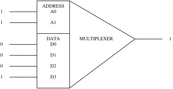
Stewart Wilson applied the classifier system to learning of a Boolean function

[13]. The classifier system learned a six-line multiplexer. The multiplexer function is

depicted schematically in Figure 2.1. Six signal lines come into the multiplexer. The

signals on the first two lines (the address or A-lines) are decoded as an unsigned binary

integer. This address value is then used to indicate which of the four remaining signals

(on the data or D-lines) is to be passed through to the multiplexer output. In Figure 2.1,

the address signal 11 decodes to 3, and the signal on data line 3 (signal = 1) is passed

through to the output (output = 1). Initially, the multiplexer function is not known by the

classifier system. Every time the input comes to the address line, the system tries to

output the correct output. When the output is correct, the system receives an appropriate

reward. As the system iterates, the classifier system learned the multiplexer and decoded

(24)

Figure 2.1: A Six-bit Multiplexer Function2

These two were some of the most successful applications of classifier system [11].

GBML such as classifier systems are applied to various fields, such as medicine, business,

or computer science. Classifier systems are used in arbitrary environment as seen in the

Goldberg’s application of classifier system to natural gas control. Such a dynamically

changing environment involves a certain level of complexity. Classifier system interacts

with such an environment with a large number of requirements, and learns to increase its

performance by processing many representation of knowledge with its mechanisms. Such

classifier system is often applied to fields where a lot of complex tasks are involved. ADDRESS

A0

A1

DATA D0

D1

D2

MULTIPLEXER

D3 1

1

0

1

2

(25)

Chapter 3: An Intensive Study on Classifier System

My thesis project was on applying the classifier system to database design. The

focus on my project was on the learning process of the classifier system. A precursor of

my project was an intensive study on the classifier system. In this chapter, the details of

classifier system are presented.

Classifier system, or learning classifier system, is the most common architecture

of genetics-based machine learning systems (GBML). Classifier system and learning

classifier system are often used interchangeably. Throughout this thesis, classifier system

is used for the term of the architecture. Classifier system learns syntactically simple string

rules called classifiers to guide its performance in an arbitrary environment [11].

Classifier system has three components: the rule and message system, the apportionment

of credit system, and the genetic algorithms.

3.1 Genetics-Based Machine Learning

The theoretical foundation of GBML was established by John Holland [14].

Holland studied natural adaptive system and its environment. He investigated whether it

is possible to formulate some key hypotheses and problems from relevant parts of

biology. He outlined how artificial systems can generate procedures enabling them to

adjust efficiently to their environments rigorously as natural biological systems. GBML

borrows the idea of genetics, the genetic properties of features of an organism. Such

GBML uses the genetic search called genetic algorithms, as their primary discovery

(26)

3.2 Genetic Algorithms

Genetic algorithms are search algorithms based on the mechanics of natural

selection and natural genetics [11]. They combine survival of the fittest among string

structures with a structured yet randomized information exchange to form a search

algorithm with some of the innovative flair of human search. Genetic algorithms have

two goals. One is to abstract and rigorously explain the adaptive processes of natural

systems. The other is to design artificial intelligence software that retains the important

mechanics of natural systems. If higher levels of adaptation can be achieved, existing

systems can perform their functions longer and better. Features for repair,

self-guidance, and reproduction are the rule in biological systems. The secrets of adaptation

on natural systems can be studied from natural biological systems. Genetic algorithms

have a power to adaptively interact with an environment. Genetic algorithms also have

robustness.

3.2.1 Robustness of Genetic Algorithms

Genetic algorithms came out with a central theme, robustness. The search is

robust if the balance between efficiency and efficacy necessary for survival in many

different environments [11]. Traditionally, there were three main types of search

methods: calculus-based, enumerative, and random. Genetic algorithms are more robust

search method, compared to the three traditional search methods.

Calculus-based methods are subdivided into two classes: indirect and direct. The

indirect methods seek local extrema by solving the usually nonlinear set of equations

resulting from setting the gradient of the objective function equal to zero. On the other

(27)

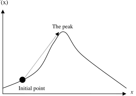
direction related to the local gradient. For example, the objective may be to find the peak

of a mountain as depicted in Figure 3.1. Indirect methods start finding the peak by setting

the initial points with slope of zero in all directions. Direct methods climb the function in

the steepest direction. Both of them successfully find the peak of the mountain. However,

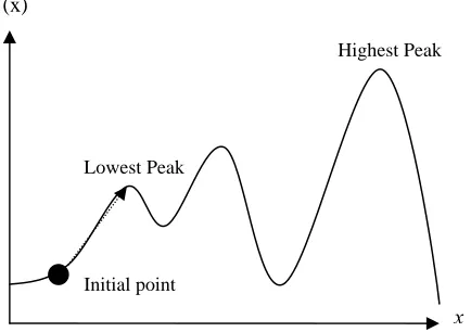
when the mountain has multiple peaks as depicted in Figure 3.2, these methods do not

always find the highest peak, since their search relies on the local best in a neighborhood

of the current point. The calculus-based methods rely on the derivatives of local and it is

hard to find the maximum value always, and thus they are not robust.

f (x)

x

Initial point

The peak

(28)

Figure 3.2: A Mountain with Multiple Peaks f (x)

x

Initial point Lowest Peak

Highest Peak

Enumerative search method is straightforward. Given a finite search space, it

enumerates all the function values at every point, one at a time. The simplicity is very

attractive and the approach is very human-like. When the number of possible solutions is

small, then this method can be used. However, many practical spaces are too large to

search one at a time. In terms of efficiency, the method is not meeting the robustness.

Random search started attracting researchers as the shortcomings of

calculus-based and enumerative methods were recognized. In random search, the possible

solutions are randomly picked. The search ends when the function value reaches the

specified value by a user. Unfortunately, random search method is expected to do no

better than enumerative method, and thus lacking in efficiency [11].

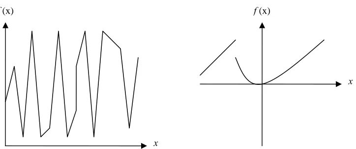
These three traditional search methods are not robust search methods. The real

world problem spaces are discontinuous, noisy, and vast multimodal. There are many of

such functions as depicted in Figure 3.3. With calculus-based search, the result may not

(29)

efficient. Genetic algorithms differ from these methods in the following search

procedures:

1. The algorithms work with a coding of the parameter set, not the parameter

themselves.

2. The algorithms search from a population of points, not a single point.

3. The algorithms use payoff of objective function information, not derivatives or

other auxiliary knowledge.

4. The algorithms use probabilistic transition rules, not deterministic rules.

Genetic algorithms are theoretically and empirically proven to provide robust search in

complex spaces [11]. The organization of the algorithms borrows the idea of natural

selection described by Charles Darwin, and the operators of the algorithms have a close

link to the theory.

f (x)

x

f (x)

x

Figure 3.3: Noisy and Discontinuous Functions

3.2.2 Natural Selection

Darwin wondered about the origin of species and the evolution of organic living

(30)

same genus. He thought that all these results follow inevitably from the struggle for life.

Darwin introduced the term, natural selection [15], in 1859 and theorized about the

evolution. Natural selection is a principle that states as follows: “Owing to this struggle

for life, any variation, however slight and from whatever cause proceeding, if it be in any

degree profitable to an individual of any species, in its infinitely complex relations to

other organic beings and to external nature, will tend to the preservation of that individual,

and will generally be inherited by its offspring. The offspring, also, will thus have a better

chance of surviving, for, of the many individuals of any species which are periodically

born, but a small number can survive.” Living things reproduce. Organic living things are

subject to a strict natural environment. Living things that have adapted to the

environment have a higher chance to survive. Living things mutate themselves to survive

the environment, and the mutation is inherited by the reproduced successors. Genetic

algorithms have operators which are artificial versions of natural selection: reproduction,

crossover, and mutation.

3.2.3 Reproduction

Reproduction in genetic algorithms is a process in which individual strings are

copied according to their objective function values, f. Biologists call this function the

fitness function. The value indicates how much the individual is fitting to the

environment for survival. We can think the function f as the profitability or goodness that

we want to maximize. As stated in Section 3.1, genetic algorithms work with a coding of

the parameter set and search from a population of points. The parameter set is coded as a

(31)

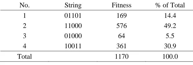
Let’s consider an example population having four strings of five-digit binary

numbers as depicted in Table 3.1. The objective function value is as follows:

2

( )

f x =x , where 0≤ ≤x 3 . 1

For example, in row 4 of the population, the value of f is with the objective

function equation. Other strings also have the fitness values according to the objective

function. In reproduction, genetic algorithms pick some strings to generate offspring for

the next generation according to their fitness function values. Then the reproduction

process replaces the strings having worst fitness values with the newly created strings

from the picked ones. Thus, the members who have higher fitness values tend to survive;

those members are reproduced and inherited by the offspring.

2

19 =361

No. String Fitness % of Total

1 01101 169 14.4

2 11000 576 49.2

3 01000 64 5.5

4 10011 361 30.9

Total 1170 100.0

Table 3.1: Example of Four Strings3

The percentage of the population total fitness is also shown in Table 3.1. In

genetic algorithms, a weighted roulette wheel by the percentage is used. Figure 3.4 shows

such a roulette wheel. The roulette wheel is a tool used to decide who to select to

generate new strings of offspring. To pick the offspring for the next generation, the

roulette wheel is turned. In this weighted wheel, the string No.1 has 14.4 percent of

3

(32)

probability to be picked for the next generation. The string No.2 has 49.2 percent of

probability, and thus has the highest probability to be picked for the next generation. In

this way, more highly fit strings have a higher number of offspring in the succeeding

generation. During the reproduction, picked strings are mated at random, and then a

crossover may proceed on each pair.

Figure 3.4: Roulette Wheel for Reproduction4

1

2 4

3

14.4%

49.2% 5.5%

30.9%

3.2.4 Crossover

The crossover operation is done as follows: an integer position k along the string

is selected uniformly at random between one and the string length less one [1, l – 1]. Two

new strings are created by swapping all characters between the positions k + 1 and the

length l inclusively. For example, consider the following mated strings A1 and A2 with a

value 4 for the k:

4

(33)

A1 = 0 1 1 0 | 1

A2 = 1 1 0 0 | 0

The character | is a separator and put at the position dividing the string. Here, the

swapping happens at the 5th character for each string. The resulted strings are as follows:

A’1 = 0 1 1 0 0

A’2 = 1 1 0 0 1

In these offspring, the characters before the position 4 are not swapped. The last element

of the string is modified by the swapping. The 0 of the A2 replaced the 1 of A1. The 1 of

A1 replaced the 0 of A2. Crossover happens in this way on each pair of the mated strings.

Each string has notions of what is important to be fitted in the environment. The

pairs picked during the reproduction are believed to have high-quality such notions. For

the binary example, the strings with high-quality notions are the ones who have 1 at the

first element. According to the objective function, to be fitted, the strings have to

maximize the fitness values by having 1s at lower positions, since the exponent increases

as the position goes to the left in the strings of binary representation. Such strings are

considered to be fitted to this example environment. The crossover operation performs

the exchange of high-quality notions between relatively fitted strings. Just as humans

borrow ideas that worked well in the past, crossover operation trades such information

between strings. When we notice a new idea, our performance sometimes gets better.

Crossover is an operation of such an information exchange. The strings with low fitness

values may get a chance to have new notions by exchanging information with other

relatively fitted strings during the crossover operation. Following the reproduction and

(34)

3.2.5 Mutation

Mutation is the occasional random alteration of the value of a string position.

Suppose there is the following string A:

A = 0 0 1 0 1

Mutation randomly picks the position. Let’s suppose the first element of the string is

mutated. The alteration is between 0 and 1 in the binary example. Since the A has 0 at the

first element, the value is altered to 1 as follows:

A’ = 1 0 1 0 1

Mutation prevents from losing some potentially useful genetic material, such as

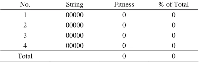
the notion that lower positions with value 1 increases the fitness value. Consider an

example of Table 3.2. There are four strings again, but each string has 0s for all the

elements, and thus all have the fitness value 0. In this case, reproduction and crossover do

not have any effect. Mutation takes place so that some strings will have new useful notion.

1 00000 0 0

2 00000 0 0

3 00000 0 0

4 00000 0 0

Total 0 0

Table 3.2: Four Strings with 0 Fitness Value

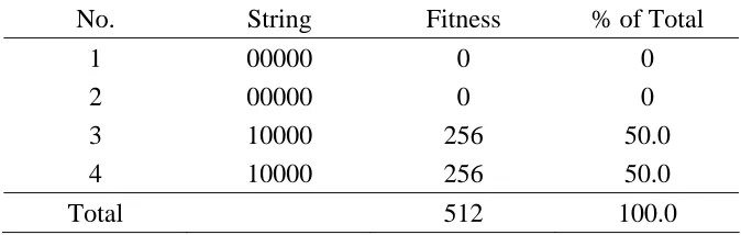
Suppose that No.1 and No.2 are picked and mated during the reproduction and

crossover. They do not affect in any way. Thus, we have two newly generated offspring

(35)

no effect. Suppose a mutation happens on the offspring, at the first element of the strings,

then we get the following:

A1’ = 1 0 0 0 0

A2’ = 1 0 0 0 0

Then, let’s replace these with strings No.3 and No.4. The table change as in Table 3.3

with the new offspring. The mutation operation provides a means to inject a new notion

to the strings. Therefore, the operator is useful when no strings have good notions to

increase the performance in the environment.

These are the operators that genetic algorithms perform. These three operators are

computationally powerful and applied to many search problems. Within the strings that

they process, there are always similarities. Strings that have relatively high fitness values

share their particular similarities; strings that have relatively low fitness values also share

their particular similarities. Genetic algorithms see these similarities in the strings and

those similarities help genetic algorithm to search. The similarity is called similarity

templates or schemata.

1 00000 0 0

2 00000 0 0

3 10000 256 50.0

4 10000 256 50.0

Total 512 100.0

(36)

3.2.6 Similarity Templates (Schemata)

Genetic algorithms are advised by the similarity templates, or schemata. A

schema [16] is a similarity template describing a subset of strings with similarities at

certain string positions. Let’s consider strings over the ternary alphabet {0, 1, *}. The

character * is a “don’t care” symbol. A schema matches a particular string if at every

location in a schema a 1 matches a 1 in the string, a 0 matches a 0, or a * matches either.

For example, if there are five strings {10000, 00000, 11100, 00001, 01110}, a schema

*0000 matches two strings {10000, 00000}. *11** will match {11100, 01110}.

Sometimes, genetic algorithms are more interested in these similarity templates, rather

than the strings themselves. This is because these similarities describe the traits of highly

fitted or badly fitted strings. These schemata of short-defining-length are propagated

generation to generation by giving exponentially increasing samples to the observed best.

This is formally stated in what is called schema theorem.

3.2.7 Schema Theorem (Fundamental Theorem of Genetic Algorithms)

Schema theorem states that short, low-order, above-average schemata receive

exponentially increasing trials in subsequent generations [11]. A schema has two

properties: schema order and defining length. The order, denoted by o(H), is the number

of fixed positions. The defining length of a schema H, denoted by δ(H), is the distance

between the first and last specific string position. For example, for a schema 011**1*, the

order is 4 and the defining length is 5. For a schema 0******, the order is 1 and the

defining length is 0. Schemata and their properties are interesting notational devices for

rigorously discussing and classifying string similarities. They provide the means to

(37)

In the reproduction, the schema theorem states that, a particular schema grows as

the ratio of the average fitness of the schema to the average fitness of the population.

Suppose that at a time t, there are m examples of a particular schema H contained in the

population A(t). Then m is written as follows:

( , )

m m H t= .

A string Ai gets selected with the following probability pi:

/

i i j

p = f

∑

f .

For each representative of H, there will be n p∗ _i copies in the population A of size n.

Therefore, at time t +1, there is the following number of examples of a schema H:

1 2

( , 1) ( ... _k) /

m H t+ = ⋅n f + f + + f

∑

f_j, where 1…k are the representatives of H.

The equation can also be written as follows:

1 2

( , ) ( ... ) / ( , )

( , 1) k

j

n m H t f f f m H t m H t

f

⋅ ⋅ + + +

+ =

∑

.

Thus:

( , 1) ( , ) ( , ) / _j

m H t+ = ⋅n m H t f H t⋅

∑

f , where f H t( , ) is the average fitness of

the strings representing schema H at time t. The average fitness of the entire population is

written as follows:

/

j f =

∑

f n.

Therefore, the m at the time t + 1 can be written as follows:

( ) ( , 1) ( , ) f H

m H t m H t

f

+ = .

This equation states that schemata with fitness values above the population average will

(38)

fitness values below the population average will receive a decreasing number of samples.

During the reproduction, we have this equation as a property.

Crossover disrupts schema sometimes when the separating point is in the defining

length of a schema. Thus we have to deal with the probability that a particular schema

survives during the crossover. Crossover survival probability is defined as follows:

( ) 1 1 s H p l δ ≥ − − .

This is because a schema tends to be disrupted whenever a site within the defining length

is selected from the length l – 1 possible position. If crossover is itself performed by

random choice, for example, with probability pc at a particular mating, the survival

probability is in the expression:

( ) 1 1 s c H p p l δ ≥ − ⋅ − .

Therefore, with reproduction and crossover, considering they are independent, the

following equation is given:

( ) ( )

( , 1) ( , ) 1

1

c

f H H

m H t m H t p

l f δ ⎡ ⎤ + ≥ _⎢ − ⋅ _⎥ − ⎣ ⎦.

With reproduction and crossover, schema H grows or decay depending on whether the

schema is above or below the population average and whether the schema has relatively

short or long defining length.

The mutation operator is the random alteration of a single position with a

probability pm, thus a single position survives at the probability 1 – pm. In order for a

schema H to survive, all of the order of schema have to survive. Therefore, the

(39)

.

( )

(1− pm)o H

For small values of pm (pm << 1), the schema survival probability is approximated by the

following expression:

1−o H p( ) _m.

The three operators of genetic algorithms are quantitatively defined as above. The

concluded equations are given as follows:

( ) ( )

( , 1) ( , ) 1 ( )

1

c m

f H H

m H t m H t p o H p

l f δ ⎡ ⎤ + ≥ _⎢ − ⋅ − _⎥ − ⎣ ⎦.

A particular schema H receives an expected number of copies in the next generation

under reproduction, crossover, and mutation as given in this equation. Also, short,

low-order, above-average schemata receive exponentially increasing trials in subsequent

generations. This conclusion is defined as schema theorem5, or fundamental theorem of

genetic algorithms. The following section shows an example of genetic algorithm

operations for a knapsack problem, where some schemata are processed as concluded in

the schema theorem.

3.2.8 A Simple Genetic Algorithm for a Knapsack Problem

Knapsack problem is one of NP-hard problems [17]. Genetic algorithms are often

applied to this kind of complex problems to search the space. Knapsack problem is

defined as follows:

We are given an instance of the knapsack problem with item set N, consisting of n

items j with profit pj and weight wj, and the capacity value c. Then the objective is

5

(40)

to select a subset of N such that the total profit of the selected items is maximized

and the total weight does not exceed c.

The problem is formulated as follows:

maximize 1 n j j j p x =

∑

subject to ,

1 n

j j j

w x c

=

≤

∑

xj∈{0,1},j=1,...,n.

In this section, the genetic algorithms deal with the following particular instance:

There are a water bottle, a pan, a ring, a camcorder, and a laptop. These are single

items, and thus the genetic algorithm can not choose to put more than one item of

the same item in the knapsack. The profit and weight of each item is given in

Table 3.4. The capacity limit is 50. The genetic algorithm has to not only

maximize the total profit, but also choose items carefully so that total weight of

the items does not exceed the capacity limit.

Water Bottle Pan Ring Camcorder Laptop

Weight 5 30 1 10 20

Profit 1 2 40 10 20

Table 3.4: Weight and Profit of the Items for a Knapsack Problem

The genetic algorithm has to deal with 128 combinations, in addition to the capacity limit.

The combinations can be represented in binary. The example is in Figure 3.5. Here, the

(41)

The string is 11010 and the total weight and the total profit value are calculated as

follows:

(Total Weight) 11010 1 5 1 30 0 1 1 10 0 20= ∗ + ∗ + ∗ + ∗ + ∗ =45

(Total Profit) 11010 1 1 1 2 0 40 1 10 0 20 13= ∗ + ∗ + ∗ + ∗ + ∗ =

In this solution, the total weight is within the capacity, but the profit could have been

better. The example genetic algorithm works with this binary representation of the

solution space.

Figure 3.5: An Example Binary Representation of the Strings in a Knapsack Problem

Table 3.5 shows the processing of strings and schemata together by the genetic

algorithm for two generations. There are four strings which are randomly generated in the

initial population. They are the first generation of the population. The total weight and

profit for each string are calculated by the functions in the table. The total weight of the

string No.1 is exceeding the capacity limit of 50. Such strings are given a value 0 for the

profit.

1 1 0 1 0

Water Bottle

(42)

String Processing String No. Initial Population (Randomly Generated) Total weight w 1 n j j j w x =

∑

Total Profit f 1 n j j j p x =

∑

Probability that ith String is

Selected i f f

∑

Expected count (from Roulette Wheel) i f f Actual count (from Roulette Wheel)

1 0 1 1 0 1 51 0 0 0 0

2 1 1 0 0 0 35 3 0.03 0.14 1

3 0 0 1 1 0 11 50 0.60 2.38 2

4 1 0 0 1 1 35 31 0.37 1.48 1

Sum 84 1.00 4.00 4.0

Average 21 0.25 1.00 1.0

Max 50 0.60 2.38 2.0

Schema Processing

Before Reproduction

String Representatives Schema Average Fitness ( )

f H

H1 1 1 0 * 0 2 3

H2 * 0 1 * * 3 50

Table 3.5: String and Schema Processing by Genetic Algorithms for a Knapsack Problem

String Processing Mating Pool After

Reproduction Mate (Randomly Selected) Crossover Site (Randomly Selected)

New Population Total Profit f (Cross Site At the

Symbol “|”) 1 n j j j p x =

∑

0 0 1 | 1 0 2 3 0 0 1 0 0 40

1 1 0 | 0 0 1 3 1 1 0 1 0 13

0 0 1 1 | 0 4 4 0 0 1 1 1 70

1 0 | 0 1 1 3 2 1 0 1 1 0 51

Sum 174

Average 43.5

Max 70

Schema Processing

After Reproduction After All Operators Expected Actual Count String

Representatives

Expected Count of Strings of a

particular Schema Actual Count String Represen-tatives Count of Strings of

a

particular Schema

0.14 1 2 0.09 1 2

2.38 2 1,3 2.98 3 1,3,4

(43)

The result of the roulette wheel matters in the reproduction. Out of four turns, the

string No.3 is picked twice and chosen to be the offspring. The offspring replaces the

worst string No.1, and resulting strings are as in the column of the mating pool. Those are

the result of reproduction. The crossover takes place on these. The mate and separating

point are determined by random choice. The result of the crossover produces the new

population. As seen in the table, the sum of the profit is increased.

What would be the bad or high-quality notion? The bad strings would be the ones

that have pan, since the pan is relatively heavy and not profitable. Clearly, the ring gives

high profit. Therefore, the strings having 1 at the third position would be good ones.

Example schemata having such notions are given as H1 and H2 in the table. H1 is a

schema having the bad notion, and the H2is the schema having the good notion. The H2

particularly increases according to the schema theorem. In the initial population, No.3 is

the string representing the schema. Therefore the value off H( ₂)is 50. According to the

schema theorem, we can expect to have m f H⋅ ( ) / f copies of the schema during the

reproduction. Therefore, the m for H2 at time t +1 can be calculated as follows:

2

( , 1) 1 50 / 21 2.38

m H t+ = ⋅ = .

In Table 3.5, two strings No.1 and No.3 of the schema in the population after

reproduction can be seen. The average of the fitness values of the strings in the mating

pool is 33.5. Therefore, we can calculate the m as follows:

.

2

( , 1) 2 50 / 33.5 2.98

m H t+ = ⋅ =

After the crossover operation, the number of strings representing the H2 is 3 (No.1, No.3,

and No.4). Whereas the H2 increases its number of strings, H1 does not. The expected

(44)

This section showed the example of genetic algorithms with a particular instance

of knapsack problem. The genetic algorithms usually work with a large number of strings

representing the solution space. Some strings representing high-quality notions are

expected to increase. By repeating the generation of offspring, the genetic algorithms

give the solutions in the form of strings, which get better and better increasing the fitness

values of each. Genetic algorithms are computationally powerful and provide means to

search. Such genetic algorithms are used as a component in classifier system, where the

strings are called classifiers.

3.3 Components of Classifier System

A Classifier system is a machine learning system that learns syntactically simple

string rules, called classifiers [11]. The classifiers guide the performance of classifier

system in an arbitrary environment. A classifier system consists of three main

components:

1. Rule and message system

2. Apportionment of credit system

3. Genetic algorithm

A classifier system is depicted in Figure 3.6. The information of environment comes to

the system through detectors. The information is decoded as message by the detectors.

Classifiers react to the environmental message. Classifiers are the thought of the system

about the environment. Based on the classifiers, the system takes actions to environment

through the effectors. When the action of the system is good, the environment gives

(45)

to understand what is good or bad by receiving such a reward. This method is called

reinforcement learning [18]. Through these components, classifiers, and reinforcement,

the system learns the environment. The objective for the system is to learn the

environment and improve the actions. The information flows from the detectors to

effectors. The rule and message system helps the flow in the classifier system.

Environment 10#: 111 00#: 000 101 000 111 Detectors Action Information Reward

Apportionment of Credit System & Genetic Algorithm Learning Classifier System

0 1 1 Message Effectors 1 1 1 Classifiers

Figure 3.6: A Learning Classifier System Interacting with its Environment6

3.3.1 Rule and Message System

The rule and message system of a classifier system is a special kind of production

system [19]. The production system has the following form:

if <condition> then <action>. 6

(46)

When t tion is fired in a typical production system. The

he l indicates the length. For example, a message of a length 3 would be a 110. The

f

ssifiers

e syntactically simple string rules. The classifier has the following

ntax:

essage>.

e where a wild card character (#) is

hen t an environmental message, the classifier reacts. For

he condition is satisfied, the ac

rule and message system employs this form, which is powerful and convenient. The

message and classifiers are structurally friendly with this form. If limited to a binary

alphabet, the message has the following syntax:

<message> ::= {0, 1}l.

T

message is used as the environmental message causing the system to react, and a part o

classifiers.

3.3.2 Cla

Classifiers ar

sy

<classifier> ::= <condition> : <m

The condition is a simple pattern recognition devic

added to the underlying alphabet:

<condition> ::= {0, 1, #}l.

W he condition is matched by

example, the four-position condition #01# matches an environmental message 0010, but

it does not match an environmental message 0000. When the classifier’s condition is

matched, the classifier becomes a candidate to send its message for the next step. When

multiple conditions are matched to the environmental message, one classifier is picked

from them. The choice is done by the apportionment of credit system, called bucket

(47)

3.3.3 Apportionment of Credit System: Bucket Brigade

Classifiers are ranked by its strength. The strength is determined by the reward

point that classifiers acquired from the environment. When multiple classifiers are the

candidates to post the message for the next step, the rank by their strength has an effect to

the pick. The bucket brigade has two components: an auction and a clearinghouse. When

the multiple classifiers are matching, then auction takes place for them. A fish market

may be a good analogy for the auction. Buyers from restaurants are the classifiers while

the fish is the environmental message. The strength may be the money that the buyers

have. The buyers may be interested in particular fish. The salespeople or fishermen sell

the fish one by one during auctions. They name a fish, and some of the buyers react to it.

Some buyers may raise their hand and tell the seller the bidding price. Thus, they have to

compete. At the end, the highest bidder wins and the fish is taken by the winner.

Classifiers also compete with other classifiers who matched to the environmental

message. The clearinghouse manages the payment keeping a record of those who bid and

those who must pay.

3.3.4 Genetic Algorithms in the Classifier System

Genetic algorithms take a role to inject new, possibly better classifiers into the

classifier system. Every time an environmental message comes to the system, there is

single winner classifier from the population and it takes an action to the environment.

Winner classifiers receive reward value from an environment when their actions are

correct. The classifier system learns if the performance increases as it experiences the

environment. Genetic algorithms replace some of the classifiers to increase the

(48)

algorithms reproduce stronger classifiers, and exchange information between classifiers,

(49)

Chapter 4: Implementation of a Classifier System in Java

I implemented a classifier system in Java programming language. The system

consists of about 30 Java classes. NetBeans is chosen as the IDE, since it provides a good

control for GUI components in the development processes. Some class diagrams

presented in this chapter are generated by NetBeans. In this chapter, some design and

implementation features of the classifier system are presented: requirements, input and

output, data structures, class diagrams, knowledge given to the system and reward

functions, and some source codes with actual operations over the classifiers. How

database schemas can be represented as classifiers, and how those classifiers are

processed in the framework of classifier system are shown.

4.1 Requirements

The first requirement is to implement the classifier system, which can represent

database schemas as its classifiers, and process those in the architecture. The classifier

system has powerful mechanisms to process classifier strings with robust genetic

algorithms as the search method. Classifiers of database schemas react to environmental

messages. Then, the matching schemas compete in an auction. The winner schema is

evaluated and receives a reward value by the reinforcement mechanism. Enabling the

processes of the classifiers in those mechanisms is the first requirement that the system

should be able to do.

Following the implementation, the learning is the main requirement for the

(50)

some may be bad. The classifier system is given some basic knowledge about database

design so that it will think what is good and what is bad. For the learning, the task T is to

pick the better one among many candidates. The performance P is determined by whether

the choice gets better as it experiences the environment E, which is doing database design

by itself. When the system stops, the system prints the strongest classifiers of each

database schema for the entity set. Every time the system experiences the database design,

it ranks the classifiers by the strength. The classifier system increases the strength of

good classifiers and decreases the strength of bad classifiers according to the knowledge.

4.2 Input and Output

Figure 4.1 shows an example input. The classifier system takes a conceptual

schema, which is a set of entity sets with the primary-key and possible non-primary key

attributes. The classifier system will randomly generate hundreds or thousands of

combinations of the attributes for each entity set. Those are represented as classifiers and

are the candidates for the final schemas. In addition, the system takes mapping

cardinalities between the entity sets. This mapping cardinality shows relationship sets and

the cardinality, such as one-to-one or many-to-many. The relationship sets are limited to

(51)

Figure 4.1: The Input to the Classifier System

Figure 4.2 shows the system tab with a pane showing the current input, a result

pane, and a plot pane to analyze the learning. The result pane is to print the strongest

classifiers for each entity set when the system completes. The strongest classifiers are the

database schemas chosen as the best by the system when it stops. The plot is to count the

number of classifiers with certain strength values at a certain iteration time point. With

the plots, the increase and decrease of the strength can be seen. These are the output of

(52)

Figure 4.2: System Tab with the Output

4.3 Data Structures

In this section, some important data structures such as classifiers, environmental

message, and population are introduced with the syntaxes. Classifiers are the main data

structure, which are involved in almost all the operations in the classifier system.

Environmental message triggers the operations of classifier system. Population maintains

(53)

4.3.1 Classifier

Classifiers represent database schemas. The classifier system randomly generates

a large number of such classifiers for every entity set, and all of those are the candidates

and have a chance to be printed at the result pane when the system stops. The classifier is

named as ClassType in the program as in Figure 4.3. Each classifier is programmatically

structured this way. The classifier has its condition and message part (action) as in the

syntax of classifier. The strength is the value indicating how well the classifier is doing in

the environment. The bid is the value that classifiers bids during the auction. The value of

matchflag indicates if the instance of the classifier is matching to the environmental

message.

Figure 4.3: The Declarations of ClassType

4.3.2 Environmental Message

Environmental message is the same as the condition part of the classifier. Thus

the environmental message has the following syntax:

<environmental message> ::= <condition>.

The environment gives the value of the condition of a classifier, and some classifiers with

(54)

condition react to the environmental message and compete. Population is another data

structure maintaining classifiers and the record for who is matching or not matching.

4.3.3 Population

Population is represented as a PopType class in the program as in Figure 4.4. The

class maintains all the classifiers in a class named ClassArray. The nclassifier is the size

of classifiers. The variables from pgeneral to ebid2 are used in the process of the auction

and genetic algorithms. The initialstrength is the strength values given to all the

classifiers when they are initially generated. The rest of the variables are to maintain the

statistical information, such as the max strength value among classifiers.

Classifier System Learning of Good Database Schema

ScholarWorks@UNO

ScholarWorks@UNO

Classifier System Learning of Good Database Schema

Classifier System Learning of Good Database Schema

Dedication

Acknowledgement

Table of Contents

List of Figures

List of Tables

Abstract

Chapter 1: Introduction

1.1 Applying the Classifier System to the Learning of Good Database

Schema

1.2 Organization

Chapter 2: Background

2.1 Artificial Intelligence

2.2 Machine Learning

2.3 Previous Works on Classifier System

Chapter 3: An Intensive Study on Classifier System

3.1 Genetics-Based Machine Learning

3.2 Genetic Algorithms

∑

∑

∑

∑

∑

∑

∑

∑

∑

∑

∑

3.3 Components of Classifier System

Chapter 4: Implementation of a Classifier System in Java

4.1 Requirements

4.2 Input and Output

4.3 Data Structures