Simulation of Combustion and Thermal-flow Inside a Pyroscrubber

University of New Orleans University of New Orleans

ScholarWorks@UNO

ScholarWorks@UNO

University of New Orleans Theses and

Dissertations Dissertations and Theses

8-7-2008

Simulation of Combustion and Thermal-flow Inside a

Simulation of Combustion and Thermal-flow Inside a

Pyroscrubber

Pyroscrubber

Lei Zhao

University of New Orleans

Follow this and additional works at: https://scholarworks.uno.edu/td

Recommended Citation Recommended Citation

Zhao, Lei, "Simulation of Combustion and Thermal-flow Inside a Pyroscrubber" (2008). University of New Orleans Theses and Dissertations. 863.

https://scholarworks.uno.edu/td/863

This Thesis is protected by copyright and/or related rights. It has been brought to you by ScholarWorks@UNO with permission from the rights-holder(s). You are free to use this Thesis in any way that is permitted by the copyright and related rights legislation that applies to your use. For other uses you need to obtain permission from the rights-holder(s) directly, unless additional rights are indicated by a Creative Commons license in the record and/or on the work itself.

Simulation of Combustion and Thermal-flow Inside a Pyroscrubber

A Thesis

Submitted to the Graduate Faculty of the University of New Orleans in partial fulfillment of the requirements for the degree of

Master of Science in

Mechanical Engineering

by Lei Zhao

ACKNOWLEDGMENT

I would like to show my deep thankfulness to my advisor Dr. Ting Wang for his sincere, patient and thoughtful guidance throughout my two years of study and research with him so far.

Without his innovative ideas and hard work, there will not be this thesis. It is great honor and luck of mine to have him as my advisor.

I would like to show appreciation to CII Carbon, L.L.C. for their trust, support and

funding on this research as well as the funding from the Industrial Ties Research Subprogram (ITRS) administered by the Louisiana Board of Regents.

I would also like to thank my colleague students and researchers from Energy Conversion and Conservation Center (ECCC), Armin Silaen, Jobaidur Khan, Day Benjamin, Zhang Zexuan, Dr. Dhanasekaran, Dr. Li Xianchang and so many others for their kind help and beneficial

discussions.

In the last I would like to thank my friends and family for their supports and

TABLE OF CONTENTS

List of Figures... iii

List of Tables ... v

Nomenclature... vi

Abstract... viii

Chapter 1 Introduction ... 1

1.1 Background... 1

1.2 Objectives ... 2

Chapter 2 Literature Survey... 4

2.1 Pyroscrubber ... 4

2.2 Combustion... 5

2.3 NOx... 6

Chapter 3 Modeling and Methodology ... 21

3.1 Governing Equations ... 24

3.2 Meshes ... 25

3.3 Inlet Condition ... 27

3.4 Turbulence Model ... 31

3.5 Combustion Model... 36

3.6 Radiation Model ... 44

3.7 NOx Emission Model ... 45

Chapter 4 Results and Discussions ... 52

4.1 Baseline Case... 52

4.2 Case 2: 80% Stoichiometric Air Combustion ... 63

4.3 Case 3: 150% Stoichiometric Air Combustion ... 68

4.4 Three Stage Combustion (41%, 39% and 20%) ... 74

4.5 Bottom Door Opening Cases... 79

4.6 Particle Combustion Model ... 83

Chapter 5 Conclusions ... 92

References... 97

Appendices ... 99

Appendix A: Application of FLUENT Code... 99

Appendix B: Pressure Driven Air Flow Velocity Estimate ... 123

Appendix C: User Defined Function (UDF) of Specifying the Surface Reaction Rate of a Particle.. 126

LIST OF FIGURES

Figure 1.1 Schematic of calcining process for petroleum coke ... 2

Figure 2.1 Fuel NOx mechanism ... 10

Figure 2.2 NO production associated with Fenimore prompt mechanism... 12

Figure 2.3 Combustion modification technologies for NOx control ... 15

Figure 2.4 Example of a typical over-fire air boiler... 16

Figure 2.5 Example of Low NOx Burner ... 18

Figure 2.6 (a) Low NOx burner employing air staging (above) (b) Low NOx burner employing fuel staging ... 19

Figure 2.7 Post-combustion control technologies for NOx reduction ... 19

Figure 3.1 A 3-D view of the pyroscrubber ... 23

Figure 3.2 Detailed air injections and burners ... 23

Figure 3.3 Meshes of different parts of the pyroscrubber ... 26

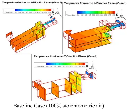
Figure 4.1 Temperature contours inside the pyroscrubber at different planes for the baseline case (100% stoichiometric air) ... 53

Figure 4.2 Representative pathlines for the baseline case (100% stoichiometric air)... 54

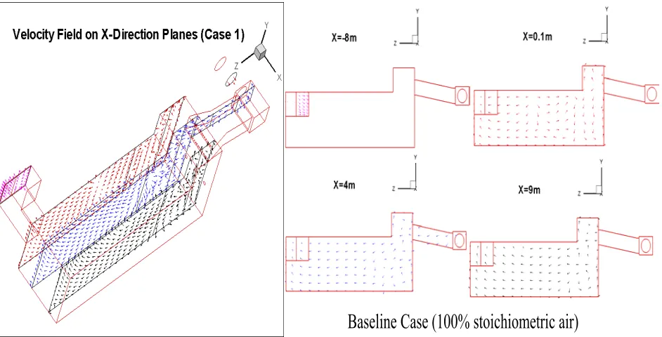
Figure 4.3 Velocity field on X-direction planes for the baseline case (100% stoichiometric air) ... 54

Figure 4.4 Velocity field on Y-direction planes for the baseline case (100% stoichiometric air) ... 55

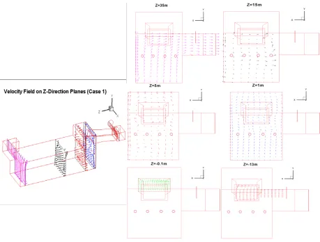
Figure 4.5 Velocity field on Z-direction planes for the baseline case (100% stoichiometric air) ... 55

Figure 4.6 Species and temperature contour plots on X-direction planes... 56

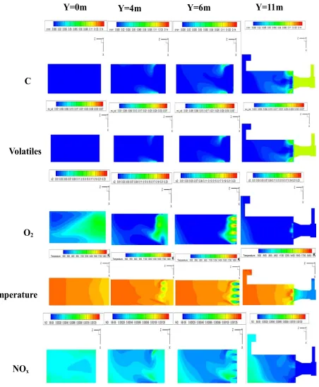
Figure 4.7 Species and temperature contour plots on Y-direction planes. ... 57

Figure 4.8 Species and temperature contour plots on Z-direction planes ... 58

Figure 4.9 Temperature contour inside the pyroscrubber for different planes for 80% stoichiometric air combustion ... 63

Figure 4.10 Velocity plots on X-direction planes for 80% stoichiometric air combustion.. 64

Figure 4.11 Velocity plots on Y-direction planes for 80% stoichiometric air combustion.. 64

Figure 4.14 Velocity plots on X-direction planes for 150% stoichiometric air combustion 70 Figure 4.15 Velocity plots on Y-direction planes for 150% stoichiometric air combustion 70 Figure 4.16 Velocity plots on Z-direction planes for 150% stoichiometric air combustion 71 Figure 4.17 Case 4 temperature contour inside the pyroscrubber for different planes with

three-stage combustion (41%, 39% and 20%)... 75 Figure 4.18 Velocity profiles for three-stage combustion in Case 5... 76 Figure 4.19 Locations for bottom doors, air injections tubes, and burner slots. ... 79 Figure 4.20 Wall temperature contours in the pyroscrubber for three bottom doors opening

case (Cases 5-7). ... 81 Figure 4.21 Temperature contour inside the pyroscrubber on different planes for coke

particle combustion with 100% stoichiometric air. ... 84 Figure 4.22 Particle pathlines for coke particle combustion (100% stoichiometric air)... 85 Figure 4.23 Species and temperature contour plots on X-direction planes for coke particle

combustion case (100% stoichiometric air). ... 86 Figure 4.24 Species and temperature contour plots on Y-direction planes for coke particle

combustion case (100% stoichiometric air). ... 87 Figure 4.25 Species and temperature contour plots on Z-direction planes for coke particle

LIST OF TABLES

Table 3.1 Kiln exit species composition summary from Zhang and Wang (2007)...29

Table 3.2 Energy release by complete combustion ...29

Table 3.3 Inlet species composition summary for 3 cases ...30

Table 4.1 Simulated results of the baseline case ...62

Table 4.2 Simulated results of 80% stoichiometric air combustion case ...67

Table 4.3 Simulated results of 150% stoichiometric air combustion case (Case 3) ...73

Table 4.4 Simulated Case 5 results of three-stage burning case ...78

Table 4.5 Simulated results of three bottom door opening cases (Cases 5-7) ...82

Table 4.6 Simulated results of particle combustion (100% stoichiometric air) ...91

NOMENCLATURE

c Concentration (mass/volume, moles/volume)

cp, cv Specific heat at constant pressure, volume (J/kg-K, Btu/lbm-°F)

Dij Mass diffusion coefficient (m2/s, ft2/s) E Total energy, activation energy (J, Btu) f Mixture fraction (dimensionless)

g Gravitational acceleration (m/s2 , ft/s2 ) H Total enthalpy (energy/mass, energy/mole) h Heat transfer coefficient (W/m2-K, Btu/ft2-hr-°F) h Species enthalpy (energy/mass, energy/mole)

h0 Standard state enthalpy of formation (energy/mass, energy/mole)

J Mass flux; diffusion flux (kg/m2-s, lbm/ft2-s)

K Equilibrium constant = forward rate constant/backward rate constant (units vary) k Kinetic energy per unit mass (J/kg, Btu/lbm)

k Reaction rate constant, e.g., k1, k-1, kf;r, kb;r (units vary)

k Thermal conductivity (W/m-K, Btu/ft-hr-°F)

kB Boltzmann constant (1.38x10–23 J/mole-K, 7.27x10-27 Btu/mole-°R)

k,kc Mass transfer coefficient (units vary) m Mass (kg, lbm)

Mw Molecular weight (kg/kgmol)

Nu Nusselt number = hL/k (dimensionless) P Pressure (Pa, atm, mm Hg, lbf/ft2) Pr Prandtl number = α/ν (dimensionless) q" Heat flux (W/m2 , Btu/ft2-hr)

R Gas-law constant (8.31447x103 J/kgmol-K, 1.98588 Btu/lbmol-°F) R Reaction rate (units vary)

Re Reynolds number ≡ UL/ν (dimensionless) S Total entropy (J/K, J/kgmol-K, Btu/lbmol-°F) s Specific entropy

s0 standard state entropy (J/kgmol-K, Btu/lbmol-°F)

Sc Schmidt number = ν/D (dimensionless) Sij Mean rate-of-strain tensor (s–1)

T Temperature (K, °C, °R, °F) t Time (s)

t thickness (m, ft)

V Volume (m3, ft3)

X Mole fraction (dimensionless) Y Mass fraction (dimensionless)

Greek Letter

α Permeability, or flux per unit pressure difference (L/m2-hr-atm, ft3/ft2-hr-(lbf/ft2))

α Thermal diffusivity (m2/s, ft2/s)

α Volume fraction (dimensionless)

β Coefficient of thermal expansion (K-1)

γ Specific heat ratio, cp/cv (dimensionless)

∆ Change in variable, final – initial (e.g., .p, .t, .H, .S, .T)

ε Emissivity (dimensionless)

ε Turbulent dissipation rate (m2/s3, ft2/s3)

η′,η″ Rate exponents for reactants, products (dimensionless)

ν Dynamic viscosity (Pa-s, lbm/ft-s) µ Kinematic viscosity (m2/s, ft2/s)

ν′,ν″ Stoichiometric coefficients for reactants, products (dimensionless)

ρ Density (kg/m3, lbm/ft3)

σ Stefan-Boltzmann constant (5.67x10–8 W/m2-K4, 1.71x10-9 Btu/hr-ft2-°R4)

σs Scattering coefficient (m–1)

τ Stress tensor (Pa, lbf/ft2)

τ Shear stress (Pa, lbf/ft2₎

τ Time scale, e.g., τc, τp (s)

ABSTRACT

The main function of a pyroscrubber in petroleum coke calcining process is to oxidize the carbonaceous contents, including hydrocarbon volatiles, of the exhaust gas from the calcination

kiln, so as to leave no more than small traces of unburned volatiles, solid carbon, ashes, or emissions (e.g. CO, NOx and SOx) in the flue gas finally discharged.

To maximize the energy recovery and reduce pollutant emission from the pyroscrubber, 3-D

computational models are developed using FLUENT to simulate the combustion and thermal-flow phenomena inside the pyroscrubber.

The results show the 3-D behavior of the flow, the reaction inside the pyroscrubber, effect of different amounts of air injection with respect to combustion efficiency, energy output and NOx

emission. A multistage burning strategy is introduced and studied and results show it

successfully cuts emission without compromising energy output. A particle combustion model with the homogeneous gas combustion model is also developed and incorporated to investigate

CO emission.

CHAPTER ONE

INTRODUCTION

1.1 Background

Petroleum coke is usually calcined in a gas-fired rotary kiln or rotary hearth at high temperatures, around 1,200 to 1,350 °C, to remove moisture, drive off volatile matters, increase the density of the coke structure, increase physical strength, and increase the electrical conductivity of the material. The product is hard, dense carbon (calcined petroleum coke) with low hydrogen content and good electrical conductivity. These properties along with the low metals and ash contents make calcined petroleum coke the best material currently available for making carbon anodes for smelting of alumina to aluminum [Bagdoyan and Gootzait, 1985].

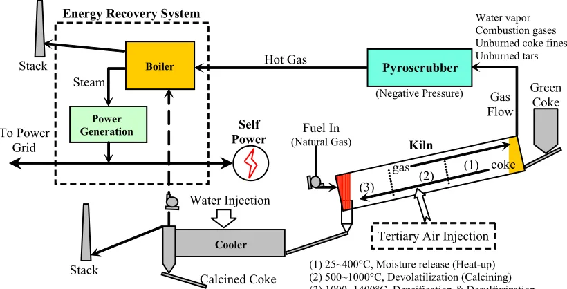
The schematic of the entire calcining processes for petroleum coke is shown in Figure 1.1. The calcination operation as mentioned above is carried out in an inclined rotary kiln where green coke is fed near the upper end. Air for combustion of volatiles is supplied at one or more locations, and burners are located at the bottom end of the kiln to provide heat at start-up and to provide supplementary heat to control the material structure and quality of the final product. Calcined coke, issuing from the lower end of the kiln, enters a rotary cooler, typically at a temperature of 1,200 oC. The coke is cooled by spraying water to quench the coke. The resultant steam, together with air drawn in through the inlet end of the cooler is drawn off through a surrounding manifold by means of a suction fan.

(1) (2) gas coke (3) Water vapor Combustion gases Unburned coke fines Unburned tars Stack Steam Kiln Pyroscrubber Fuel In (Natural Gas) Green Coke Gas Flow (Negative Pressure) Hot Gas

(1) 25~400°C, Moisture release (Heat-up) (2) 500~1000°C, Devolatilization (Calcining) (3) 1000~1400°C, Densification & Desulfurization

Tertiary Air Injection Self

Power

Water Injection Energy Recovery System

Calcined Coke Cooler Boiler Stack Power Generation To Power Grid

Figure 1.1 Schematic of the calcining process for petroleum coke

1.2 Objectives

To maximize the energy recovery and reduce pollutant emission from the pyroscrubber, more detailed information and a better understanding of thermal-flow and combustion process inside the pyroscrubber are needed. The objective of this study is to employ computational fluid dynamics (CFD) technique with the appropriate combustion model to better understand the combustion and thermal-flow phenomena inside the pyroscrubber, and investigate further the potential means to improve combustion performance and reduce emissions. The specific goals are:

1. Develop a numerical model of the pyroscrubber that simulates the thermal-flow, combustion processes. Special attention will be paid to the modeling of coke fines, combustion gases burning, and pollutant emissions.

2. Investigate flow pattern, temperature distribution, combustion process, and emission information inside the pyroscrubber.

4. Simulate and study the effect of introducing a multistage burning strategy on emission control and energy output.

CHAPTER TWO

LITERATURE SURVEY

The literature survey focuses on introducing types, functions, fundamental mechanisms

of combustion and emissions in pyroscrubbers.

2.1 Pyroscrubber

A pyroscrubber is namely a furnace burning carbon particles in a stream of waste gas, particularly from a petroleum coke calcination kiln or hearth. The combusted hot gases are

ducted through a boiler to produce steam that is used to generate electricity through steam turbines. A pyroscrubber typically comprises of a U-shaped combustion chamber having a first

passage arranged parallel with (preferably above) a second passage, so there is a reversal in gas flow direction between the two passages. The combustion chamber has an inlet to receive exhaust gases from the calcining kiln and an array of air injection inlets at the inlet end of the

first passage. A gas outlet preferably leads laterally out of the side of the structure at the outlet end of the second passage to secure an abrupt change in the direction of gas flow. The main

function of the pyroscrubber is to oxidize the carbonaceous contents, including hydrocarbon volatiles in the exhaust gas from the calcination kiln, so as to leave no more than small traces of unburned volatiles, solid carbon, ashes, or emissions (e.g. CO, NOx and SOx) in the flue gas

finally discharged. Where incandescent carbon particles are carried in an oxygen-containing gas stream, the products of its own combustion tend to increase in its immediate surroundings and

speed from the entrained particles, there is "slip" or relative movement of the particles to the gas. The reversed-flow two-passage design in the pyroscrubber construction has the advantage because the gases passing through the combustion chamber turn through 180o in

passing from the first passage to the second passage, leading to an increase in turbulence in the gas stream and in the slip between the gas and the entrained particles. This leads to increased

speed of combustion by separating the coke particles from their own combustion products. Pyroscrubbers of different designs have been employed worldwide to compete for more efficient and cleaner combustion of exhaust gases from coke calcination kilns or hearths. Known

pyroscrubbers have comprised of a long, straight combustion chamber with a large cross section to permit passage of the large volume of gases flying through with dense carbon particles. They

rely on normal flue draught for drawing in air at various locations in the combustion chamber. Supplementary air is drawn into the combustion chamber at a substantial distance from the inlet end of the combustion chamber, which results in a delay of thorough mixing of the air and the

waste gas stream to ensure a complete combustion of solid carbon particles. Consequently, the dimensions of the combustion chamber of known pyroscrubbers are rather large. Since the function of pyroscrubber-steam generator assembly is similar to the conventional coal-fired

boiler assembly, the literature search will start with boiler review.

2.2 Combustion

Combustion or burning is a complicated sequence of chemical reactions between a fuel and an oxidant accompanied by the production of heat or both heat and light in the form of either a glow or flames. In a complete combustion reaction, a compound reacts with an oxidizing

Heat CO

O

C+ ₂ → ₂ + (Eq.2.1)

In reality, combustion processes are never perfect or complete. In flue gases from

combustion of carbon (Eq.2.2) or carbon compounds (as in combustion of hydrocarbons, wood etc.) both unburned carbon (known as soot) and carbon compounds (CO (Eq.2.3) and others) will be present.

Heat CO

O

C+12 ₂ → + (Eq.2.2) Heat

CO O

CO+ 12 ₂ → ₂ + (Eq.2.3) Also, when air is the oxidant, some nitrogen will be oxidized to various, mostly harmful, nitrogen oxides (NOx). The effectiveness of combustion can be determined by analyzing the flue

gas and the amount of soot.

There are three types of fuel present in the calcining process, methane (as natural gas), solid carbon (as petroleum coke), and volatile matters (as hydrocarbons).

The complete combustion of methane and volatile matters can be presented as:

Heat O

2H CO 2O

CH₄ + ₂ → ₂ + ₂ + (Eq.2.4)

(

)

O H

Cx y z+ +y4 −z2 2 → 2 +y2 ₂ + (Eq.2.5)

2.3

NO

Control of NOx emission is a major factor in the design of a modern combustion system.

NOx emissions cause serious health issues, ranging from bronchitis to altered immune system

function. Currently, 8.5 million Americans live in countries with NOx levels higher than EPA’s

health standards prescribed. NOx also contributes significantly to environmental problems such

as acid rain and ozone depletion.

and nitrous oxide (N2O). The quantity of NOx formed depends on the three T’s: Temperature,

Time, and Turbulence.

Oxides of Nitrogen Formation:

In every circumstance where combustion occurs, the formations of nitrogen oxides (NOx)

are inevitable. From a home open fire to a coal fired power plant, NOx is formed as an undesired

product and a contributor to air pollution.

NOx is used to refer to NO and NO2. NO is the primary form in combustion products

(typically 95 percent of total NOx). NO is subsequently oxidized to NO2 in the atmosphere.

Nitrogen Oxide formation occurs through three reaction paths, each having unique

characteristics which are responsible for the formation of NOxduring combustion processes:

(1) Thermal NOx: formed by the combination of atmospheric nitrogen and

oxygen at high temperatures

(2) Fuel NOx: formed from the oxidation of fuel-bound nitrogen

(3) Prompt NOx: formed by the reaction of fuel-derived hydrocarbon fragments

with atmospheric nitrogen in an early phase of the flame front

NOx emissions do not form in significant amounts until flame temperatures reach

1810.93 K (2800o_{F). Once that threshold is passed, any further rise in temperature causes a rapid}

increase in the rate of NOx formation. Lower excess air levels (fuel rich) starve the reaction for

oxygen, and higher excess air levels (lean burn) drive down the flame temperature, slowing the

rate of reaction, hence reducing thermal NOx formation.

In the combustion of fuels that contain no nitrogen, nitric oxide is formed by three chemical mechanisms:

2. The Prompt or Fenimore Mechanism 3. The N2O Intermediate Mechanism

Thermal NOx Formation

Thermally produced NOx is the largest contributor to these types of emissions. Thermal

NOx is produced during the combustion process when nitrogen and oxygen are present at

elevated temperatures. The two elements combine to form NO or NO2. NOx is generated by

many combustion processes. It combines with other pollutants in the atmosphere and creates O3,

a substance known as ground level ozone.

The formation of thermal mechanism dominates in high-temperature combustion over a fairly wide range of equivalence ratios. Equivalence ratio is defined as the ratio of actual fuel/air ratio over the theoretical fuel/air ratio. The formation of thermal NOx is determined by a set of

highly temperature-dependent chemical reactions known as the extended Zeldovich mechanism. The principal reactions governing the formation of thermal NOx from molecular nitrogen are as

follows:

O + N2 ⇔ NO + N (Eq.2.6)

N + O2 ⇔ NO + O (Eq.2.7)

A third reaction, particularly at near-stoichiometric conditions and in fuel-rich

mixtures, contributing to the mechanism is

N + OH ⇔ NO + H (Eq.2.8)

unimportant at temperatures below 1800 K (2780oF). Compared with the time scales of fuel oxidation processes, NO is formed rather slowly by thermal mechanism; therefore, thermal NO is generally considered to be formed in post flame gases.

Fuel NOx Formation

Fuel NOx formation is a more complex process involving local concentration of oxygen

and nitrogen and is reduced by minimizing the availability of oxygen during various stages of the

combustion process. Fuel-bound NOx is generated from nitrogen compounds present in the fuel

itself. Gaseous fuels, such as natural gas or propane, are free of nitrogen compounds. However,

fuel oils and coal can contain significant amounts of fuel-bound nitrogen. During combustion, the conversion rate of fuel-bound nitrogen to NOx varies widely over a range of 20 to 70%.

During the combustion process, nitrogen-containing organic compounds present in liquid

or solid fossil fuel contributes to the total NOx formed. The fuel nitrogen is a particularly

important source of nitrogen oxide emissions for residual duel oil, coke, and coal, which

typically contain 0.3-2% nitrogen by weight. The fuel-bound NOx contribution depends on the

amount of nitrogen that is chemically bound in the fuel. The fuel NOx formation is generally

important in non-premixed combustion. The fuel NOx formation is not important in premixed

combustion applications since most fuels used in premixed combustion contain little or no bound

nitrogen.

Under the reducing conditions surrounding the burning droplets or particles, the

fuel-bound nitrogen is converted to fixed nitrogen species such as HCN and NH3. These, in turn,

percent of the bound nitrogen is typically converted to NOx, depending on the design of the

combustion equipment. With prolonged exposure (order of 100 ms) to high temperature and reducing conditions, however, these fixed nitrogen species can be converted to molecular

nitrogen and avoid the NO formation path. The fuel NOx mechanism is shown in Figure 2.2.

Fuel Nitrogen

NH3

HCN

NO

N2

NO

NO O2

O2

Figure 2.1 Fuel NOx mechanism

Prompt NOx Formation

Prompt NOx is the third and least significant NOx formation mechanism. In this

mechanism, nitrogen from combustion air reacts with hydrocarbon radicals from the fuel to form a hydrogen cyanide intermediate. The hydrogen cyanide then reacts with oxygen and nitrogen in

combustion air to form nitrogen oxide.

Hydrocarbon fragments (such as C, CH, CH2) may react with atmospheric nitrogen under

fuel-rich conditions to yield fixed nitrogen species such as NH, HCN, H2CN, and CN. These in

nitrogen-containing fuels, the prompt mechanism is responsible for only a small fraction of the

total NOx. Its control is important only when attempting to reach the lowest possible emissions.

The formation of prompt NOx is governed by a set of equations known as Fenimore

mechanism. These equations show that hydrocarbon radicals react with molecular nitrogen to

form amines or cyano compounds. The amines and cyano compounds are then converted to

inverted compounds that ultimately form NO. Fenimore mechanism is given as:

CH + N2 ⇔ HCN + N (Eq.2.9)

C + N2⇔ CN + N (Eq.2.10)

N + O2⇔ NO + O (Eq.2.11)

HCN + OH ⇔ CN + H2O (Eq.2.12)

N + OH ⇔ NO + H (Eq.2.13)

In the atmosphere, nitric oxide ultimately oxidizes to form nitrogen oxides, which

contribute to production of acid rain and photochemical smog. Production of NO associated with

F

igure 2.2 NO production associated with Fenimore prompt mechanism

Prompt NOx formation is proportional to the number of carbon atoms present per unit

volume and is independent of the parent hydrocarbon identity. The quantity of HCN formed

increases with the concentration of hydrocarbon radicals, which in turn increases with

equivalence ratio. As the equivalence ratio increases, prompt NOx production increases, passes a

peak, and finally decreases due to deficiency in oxygen.

NOx Formation From Reburning

In reburning NO mechanism, NO reacts with hydrocarbons and is subsequently reduced.

In general the mechanism is given as

CHi + NO –→HCN + products (Eq.2.14)

Three reburn reactions for temperature range 1600 ≤ T≤ 2100 K are

CH + NO –K1→ HCN + O (Eq.2.15)

CN N

NCO NH HCN

CH2

Fuel-N HNCO

NO N2

H2 OH

N2 O OH H H O2 NH2 NO O

H2O

H2

O

OH OH

OH OH H

CH2 + NO –K2→ HCN + OH (Eq.2.16)

CH3 + NO –K3→ HCN + H2O (Eq.2.17) Where K1, K2 and K3 are rate constants for the above reactions

K1 = 1 * 108 [m3 / gmol-s]

K2 = 1.4 * 106 * e-550/T [m3 / gmol-s]

K3 = 2 * 105 [m3 / gmol-s]

NOx Control

NOx control technologies currently used within the industry can be grouped into two

categories i.e. combustion modifications and post-combustion NOx control technologies. The

first addresses reduced production of NOx by making changes in the combustion process or the

fuel stream. The second involves mitigating the NOx that has been produced by the application of

post-combustion technology through the use of chemical reagents. For coal-fired applications, combustion system modifications are generally less costly and may independently result in emissions levels that satisfy regulatory requirements. Several methods are available to effectively

limit NOx formation during combustion. The optimum combustion system redesign may blend

several of these, including selected on the basis of unit capacity, fuels to be fired,and

applicable NOx reduction requirements.

For processes dominated by thermal NOx formation, time, temperature, and oxygen

availability are the primary variables affecting NOx yields. Production of thermal NOx can be

controlled by reducing the thermal loading to the combustion zone. NOx mechanisms include (1)

increasing the size of the combustion zone for a given thermal input, (2) reducing the rate of

recirculated flue gas to the combustion air to depress flame temperature and increase residence time.

Fuel NOx formation can be reduced by switching to, or co-firing with, fuel with lower

nitrogen content and/or by limiting oxygen availability during the early stages of combustion. Oxygen reduction mechanisms include reducing excess air, reducing burner stoichiometry by removing a portion of the combustion air from the burner zone and introducing this air later

through NOx or overfire air (OFA) ports (i.e. air staging), and limiting the rate that air is

introduced to the fuel during the early stages of combustion with specially designed burners.

Combustion Modifications for NOx control

Low Excess Air ---- Reducing the air supplied in the furnace lowers NOxproduction. Thermal

NOx emissions peak at leaner than stoichiometric equivalence ratios. The NOx creation rate

typically peaks at excess oxygen levels of 5-7% where the combination of high combustion

temperatures and the higher oxygen concentration act together. At both lower and higher air/fuel ratios, NOx production falls off due to lower flame temperature at high excess air levels and

lower oxygen at low air levels. Low air is achieved by changes in operating procedures, system

controls or both. The NOxreduction technique involves reducing the air supplied. Only limited

NOxreductions are possible when low air level is supplied because excessive reduction in air can

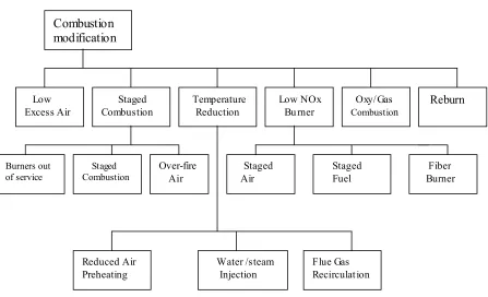
Combustion modification Low Excess Air Staged Combustion Temperature Reduction Low NOx Bu rner Oxy/Gas Combustion Reburn Burners out of service Staged Combustion Over-fire Air Staged Air Staged Fuel Fiber Burner Reduced Air Preheating Water /steam Injection Flue Gas Recirculation

Figure 2.3 Combustion modification technologies for NOx control

Staged Combustion — Staged combustion processes significantly reduce NOxemissions. In the

initial stage of combustion, the air supplied to the burners is less than the amount required to completely burn the fuel. During this stage, fuel-bound nitrogen is released but cannot be oxidized, so it forms stable molecules of harmless molecular nitrogen (N2). Other components of

the fuel are also released without being fully oxidized. These include carbon particles and carbon monoxide. By adding a second stage, in the air-fuel mixture, the carbon and carbon monoxide

can be burned, converting them to carbon dioxide.

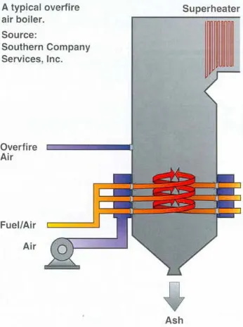
Over-fire Air — Over-fire air is the air that is injected into the furnace above the normal combustion zone. Generally when Over-fire air is employed, the burners are operated at a lower

than normal air-to-fuel ratio, which reduces NOx formation. Over-fire air, which is frequently

temperature. Figure 2.4 shows a typical over-fire air boiler.

Figure 2.4 Example of a typical over-fire air boiler (Source: Southern Company Services, Inc.)

Flue Gas Recirculation — Flue Gas Recirculation, in which part of the flue gas is recirculated to the furnace, can be used to modify conditions in the combustion zone (lowering the temperature and reducing the oxygen concentration) to reduce NOx formation. Flue Gas

Recirculation is also used as a carrier to inject fuel into a reburn zone to increase penetration and mixing.

Operational Modifications — Changing certain boiler operational parameters can create

conditions in the furnace that will lower NOx production. Examples include

burners-out-of-service (BOOS), low excess air (LEA), and biased firing (BF). In BOOS, selected

(typically the lower burners) while reducing fuel to other burners (typically the upper burners) to create staged combustion conditions in the furnace.

Low NOx Burners (LNB) — Low NOx Burners are burners designed to control the mixing of

fuel and air to achieve what amounts to staged combustion. This staged combustion reduces both

flame temperature and oxygen concentration during some phases of combustion, in turn, reduces

both thermal NOx and fuel NOx production. An example of LNB is shown in Figure 2.5 The

most common LNB types achieve lower NOx emissions by "staging" the injection of either air or

fuel in the burner region. Low NOx burners are classified as either a staged air or a staged fuel

burner. Air staging is more common. As the name implies, the staged air burner gradually

introduces combustion air to the fuel at various regions along the flame front. These regions are

typically referred to as the primary, secondary and tertiary (staged) air zones. The division of

combustion air reduces the oxygen concentration in the primary burner combustion zone,

lowering the amount of NO formed there and increasing the amount of NO-reducing agents

formed in an oxygen deficient combustion zone. Secondary and tertiary air injections complete

the combustion downstream of the primary zone, lowering the peak temperature and reducing

thermal NOx formation. Aside from the basic staged air burner, there are other variations of

staged air burners that incorporate internal recirculation of combustion products to aid in NOx

reduction. Low NOx burners are often coupled with over fire (secondary) air (OFA) injection to

assure complete combustion. Low NOx burner employing air staging and fuel staging is shown in

Figure 2.6.

Reburning — In the Reburning process, part of the boiler fuel input (typically 10-25%) is added

NOx formed in the normal combustion zone. OFA is injected above the reburn zone to complete

combustion. Thus with reburn, there are three zones in the furnace: (1) a combustion zone with

an approximately normal air-to-fuel ratio, (2) a reburn zone where added fuel results in a

fuel-rich condition, and (3) a burnout zone where OFA completes the combustion. Coal, oil, or

gas can be used as the reburn fuel.

Figure 2.5 Example of Low NOx Burner (Source: the International Energy Agency)

(b)

Figure 2.6 (a) Low NOx burner employing air staging (above)

(b) Low NOx burner employing fuel staging

(Source: The John Zink Combustion Handbook)

Post-Combustion controls for NOx reduction

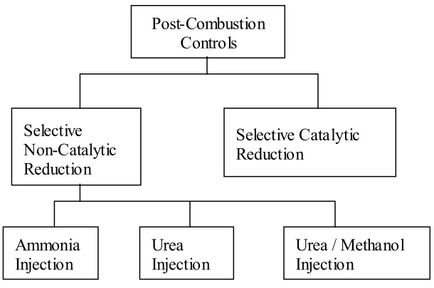
Post-combustion controls can be achieved by using selective non-catalytic reduction (SNCR) and selective catalytic reduction (SCR) as shown in Figure 2.7

Post-Combustion Controls

Selective Non-Catalytic Reduction

Selective Catalytic Reduction

Ammonia

Injection Urea Injection Urea / Methanol Injection

Selective Non-Catalytic Reduction (SNCR) — In this post control technique, a nitrogen containing additive, ether ammonia, urea, or cyanuric acid, is injected and mixed with flue gases

to affect chemical reduction of NO to N2 without the aid of catalyst. Temperature is a critical

variable, and operation within a relatively narrow range of temperatures is required to achieve

large NOx reductions.

Selective Catalytic Reduction (SCR) — In this technique, a catalyst is used in conjunction with ammonia injection to reduce NO to N2. Effective reduction depends on the temperature range

and is about 480 K to 780 K. Greater NOxreductions are possible, but the cost of NOx removal

is generally the highest of all NOx control techniques because of both the initial cost and the

CHAPTER THREE

MODELING AND METHODOLEGY

The pyroscrubber studied in this thesis is shown in Figure 3.1. Geometric information of the pyroscrubber is obtained through the blueprints of the CII Carbon Norco Plant in Louisiana.

Assumptions and simplifications are made for effective modeling and simulation. The modeled domain includes part of the calcining kiln, settling chamber, inlet duct, which connects the settling chamber with the main chamber, air injection section, main chamber, and outlet

duct,connecting the main chamber to the boiler. Details of the air injectors and the burner are shown in Figure 3.2.

The inlet of the pyroscrubber receives exhaust gases from the exit of the calcining kiln.

After completion of the calcining process inside the kiln, combustion product gases, together with unburned volatiles and coke fines are fed into the pyroscrubber through the settling chamber

and the inlet duct. Air is injected into the main chamber through two air injection sections. The first air injection section consists of 28 air injection tubes shooting at 45o from the vertical direction (Y direction). Not only is the second air-injection section, located at the burner slots

on the east wall of the main chamber, used to inject natural gas as the start-up fuel, but they also blow air into the main chamber after the ignition and start-up process. Hot product gases

exit the pyroscrubber main chamber through the outlet duct and are fed into the steam boiler to generate electricity.

1. The flow inside the pyroscrubber is three dimensional, incompressible, and turbulent.

2. Gas species involved in this study are Newtonian fluids with variable

properties as functions of temperature.

3. Buoyancy and radiation effects are considered.

4. Non-slip and adiabatic wall conditions are assumed.

CFD commercial software FLUENT (version 6.2.16) is employed to complete the

calculation process of the modeling. The simulation uses the segregated solver, which employs an implicit pressure-correction scheme. The SIMPLE algorithm is used to couple the pressure

and velocity. Second order upwind scheme is selected for spatial discretization of the convective terms and species. Lagrangian trajectory calculations are employed to model the dispersed phase of particles. The impact of particles on the continuous phase is considered as

source terms to the governing equations. After obtaining an approximate flow field of the continuous phase (gas flow in this study), particles are injected and their trajectories are calculated. At the same time, drag, heat and mass transfer between the droplets and the airflow is

calculated.

Iteration proceeds alternatively between the continuous and discrete phases. Twenty iterations in the continuous phase are conducted between two iterations in the discrete phase.

Converged results are obtained after the specified residuals are met. A converged result renders mass residual of 10-4, energy residual of 10-6, and momentum and turbulence kinetic energy

representative of the flow rate. Typically, 8000 to 12000 iterations are needed to obtain a converged result, which takes about 15~20 hours on a 10-node computer cluster of parallel computation with each node a 2.8 GHz Pentium personal computer.

Settling Chamber Outlet Duct

Main Chamber

Kiln

Inlet Duct Burners Slots

Air Injection Tubes

South Wall

North Wall West Wall

East Wall High Bay

Low Bay

Figure 3.1 A 3-D view of the pyroscrubber

3.1 Governing Equations

The conservation equations for mass, momentum and energy in general forms are shown

below.

( )

t

ρ_{+∇• =} ∂

∂ _v

(Eq.3.1)

( )

( )

( )

t

v v v

v

v _{+∇• =−∇ +∇• + +}

∂ ∂

(Eq.3.2)

( )

(

(

)

)

j j j

eff T h J v S

k p

E V E

t _+

         _{τ •} + − ∇ • ∇ = + ρ • ∇ + ρ ∂

∂ v

_∑

The momentum equations are solved with the complete three-dimensional Navier-Stokes

equations, so,τ , the stress tensor is given by

(

)



_{∇ +∇ − ∇• •} µ

=

τ v I

3 2 v

v vT v

v

(Eq.3.4) where I is the unit tensor.

In the energy equation, E is given as

2 v p h E 2 + ρ −

= (Eq.3.5)

“h” is the sensible enthalpy and for incompressible flow and it is given as

ρ + =

∑

j j

j (Eq.3.6)

∫

h (Eq.3.7)

Tref is the reference temperature, taken as 298.15 K

from the species transport reactions.

3.2 Meshes

The mesh used in this study is generated using GAMBIT (version 2.2.30). Structured

grids are employed in meshing the kiln, part of the main chamber, and the outlet duct; unstructured grids are employed for all the other parts, namely the settling chamber, inlet duct,

and part of the main chamber. All together there are 70,729 nodes, 708,418 faces and 340,800 cells. Meshes of each part are shown in detail in Figure 3.3.

Grid Sensitivity Study

A grid sensitivity study of two different mesh numbers (325,431 and 968,235) has been

performed and investigated. The computational time for the low mesh number case is about 20 hours and for the high mesh number case is about 60 hours. The temperature variation within the

whole domain lies within 50k to 150k (2.6%-7.9%). At the exit, the difference of mass weighted temperature is about 90 K (4.7%). Although the grid independency has not been achieved, for the purpose of current study, 10 % of computational uncertainty is acceptable. Therefore the mesh

Enlarged by 600%

Setting Duct

Settling Chamber

Main Chamber Outlet Duct

3.3 Inlet Condition

The composition of the pyroscrubber inlet species is complex due to the calcining and combustion process inside the kiln. Since their quantities are not subject to measurement yet, the inlet condition is prone to uncertainty. Therefore, a sound estimate of the inlet species is

critical for conducting an appropriate simulation. The inlet condition of the pyroscrubber is based on information from three sources: (a) the electric power output from the steam power plant, (b)

the computational simulation results of the rotary kiln from a previous report (Sean Zhang and Wang 2007), and (c) the model from a previous Canadian report. Detailed information from each of the three resources is provided below:

(a) According to the operation data of the steam power plant, the hot gases coming out of the pyroscrubber supply the energy for the steam power plant to generate a power output of 15MW. The overall efficiency for the steam power plant is 29.75%

(85% boiler efficiency and 35% steam turbine efficiency).

(b) From a previous report (Sean Zhang and Wang 2007), which simulates the calcining process inside the kiln, the exit species composition from the kiln is

shown in Table 3.1.

(c) From the Canadian report, the kiln feeding information is:

Green coke feed rate: 9.3 kg/s (16.74 ton/hr, here 1short ton = 2000 lbs)

5.2 % moisture 0.15 % impurities

10.2 % volatile matters (4.09 % burned in kiln and 6.11 % unburned goes into

3.72 % coke burned in kiln

9.12 % coke goes into pyroscrubber Yield: 71.61 % (mass)

To appropriately set up the inlet condition, the information from these three resources

needs to be re-examined, cross-checked, and verified. The following observations are made based upon the information from these three sources.

1. All three sources suggest natural gas is burned out inside the kiln, and it is not an

important energy source in the pyroscrubber.

2. The energy released and used for the power generation comes from two main sources: coke fines and unburned volatile matters.

3. From Table 3.1, it is noticed that the total energy generated from source (b) is not enough to sustain a 15 MW power output through the current steam power plant because coke fines entrainment from the kiln into the pyroscrubber are not

considered in the calculation of source (b). The energy deficiency between (a) and (b) is supplied by combustion of coke fines.

4. Table 3.2 shows the necessary mass flow rate of using only carbon or volatiles as the

fuel to supply the 15MW power output. Based on the calculation, it can be concluded that the majority of energy is from the coke fines rather than the volatile.

Based on the above information, the following assumptions are made in this study:

1. The green coke feed rate is 9.3 kg/s, of which 6% is moisture. After the moisture is

feed rate of the kiln is 9.3kg/s×0.94×0.08=0.6994kg/s, of which 40% (0.28 kg/s) is burned in the kiln and 60% (0.42 kg/s) goes into the pyroscrubber.

2. Coke fines are entrained into the pyroscrubber at the rate of 1.54kg/s.

3. All the other gas species feeding rates into the pyroscrubber follow the results given by report (Sean Zhang and Wang 2007).

Table 3.1 Kiln exit species composition summary from Zhang and Wang (2007)

species mass fraction mass flow rate(kg/s) standard state enthalpy (J/kgmol) energy released through complete combustion (J/kg-fuel) total energy released(MW)

N2 0.709 9.091 0 -

-CH4 0.000 0.000 -7.49E+07 -

-C 0.001 0.017 -101.268 3.28E+07 0.554 H20 0.075 0.964 -2.42E+08 -

-CO2 0.197 2.520 -3.94E+08 -

-O2 0.010 0.127 0 -

-volatile 0.008 0.099 -5.60E+07 4.12E+07 4.100 total 1.000 12.818 _- - 4.654

Table 3.2 Energy release by complete combustion

fuel

energy released through complete combustion(kJ/kg fuel)

mass flow needed for 15MW power generation(kg/s)

C 3.28E+04 1.537

Table 3.3 Inlet species composition summary for 3 cases

i nl et speci es

mass

f l ow( kg/ s) mass f r act i on

St oi chi omet r i c ai r needed ( kg/ s)

80% ai r ( kg/ s)

150% ai r ( kg/ s)

N2 9. 070 0. 622 0. 000

CH4 0. 000 0. 000 0. 000

C 1. 537 0. 105 17. 669

H20 1. 154 0. 079 0. 000

CO2 2. 159 0. 148 0. 000

O2 0. 237 0. 016 - 1. 021

vol at i l e 0. 419 0. 029 5. 719

t ot al 14. 577 0. 999 22. 366

bur ner ai r

i nj ect i on 11. 483 0. 513 11. 483 9. 186 17. 224

ai r i nj ect i on-up

5. 442 0. 243 5. 442 4. 353 8. 163

ai r -i nj ect -i on-down

5. 442 0. 243 5. 442 4. 353 8. 163

same as inlet

condition in

stoichiometric case

O2 indicates the amount of air which can be reduced due to oxygen contained in the incoming

fuel. In the Other boundary conditions of different surfaces are listed as following: 1. Inlet temperature:

a Main inlet gases: 500 K (440.33 °F). b Injection tubes air: 300 K (80.33 °F)

c Burner slots air: 300 K (80.33 °F)

2. Pressure outlet -- The outlet is defined as the constant pressure outlet. The pressure,

temperature, and species mass fraction of the mixture of the potential reverse flow are specified as follows:

a. Gas outlet: Constant pressure outlet condition, P = 1 atm

b. Temperature condition, Toutlet = 1000 K (1340.33 °F)

c. Mass fraction:

i. O2 = 0.23

ii. N2 = 0.77

3. Wall -- The walls are treated as adiabatic with no-slip velocity condition:

a. Adiabatic wall condition, heat flux = 0

b. No slip condition at the walls, u = 0, v = 0, w = 0

3.4 Turbulence Model

The standard k - ε model is employed in this study to simulate the turbulent flow due to its suitability for a wide range of wall-bounded and free-shear flows. The standard k - ε model is

ε model is a semi-empirical model with several constants, which were obtained from experiments.

All the three k - ε models have similar forms with major differences in the method of

calculating the turbulent viscosity: the turbulent Prandtl numbers and the generation and destruction terms in the k - ε equations.

The standard k - ε model is a semi-empirical model based on model transport equations for the turbulence kinetic energy (k) and its dissipation rate (ε). The model transport equation for (k) is derived from the exact equation; while the model transport equation for (ε) is obtained

using physical reasoning and bears little resemblance to its mathematically exact counterpart. The turbulence kinetic energy (k), and its rate of dissipation (ε), are obtained from the following transport equations:

( )

(

)

j k t j i i S Y G G x k x ku x k

t __+ + −ρε− +

     ∂ ∂       σ µ + µ ∂ ∂ = ρ ∂ ∂ + ρ ∂ ∂ (Eq.3.8)

( )

(

)

(

)

In these equations, Gk represents the generation of turbulence kinetic energy due to the mean

velocity gradients and the Reynolds stress, calculated as

i j ' j ' i k x u u u G ∂ ∂ ρ −

= (Eq.3.10)

Gb represents the generation of turbulence kinetic energy due to buoyancy, calculated as

i t t i b x T Pr g G ∂ ∂ µ β

= (Eq.3.11)

where Prt is the turbulent Prandtl number and gi is the component of the gravitational vector in

β is the coefficient of thermal expansion and is given as P T 1       ∂ ρ ∂ ρ − =

β (Eq.3.12)

YM represents the contribution of the fluctuating dilatation in compressible turbulence to the

overall dissipation rate, and is given as

2 t

M 2 M

Y = ρε (Eq.3.13)

where Mt is the turbulent Mach number, given as

2 t

a k

M = (Eq.3.14)

where a = (γRT)0.5 is the speed of sound.

The turbulent (or eddy) viscosity, µt, is computed by combining k and ε as

ε ρ =

µ_t C_µ k2 (Eq.3.15)

C1ε, C2ε, Cµ, σk and σt are constants and have the following values

C1ε = 1.44, C2ε = 1.92, Cµ = 0.09, σk = 1.0, and σt = 1.3

These constant values have been determined from experiments using air and water for

fundamental turbulent shear flows including homogeneous shear flows and decaying isotropic grid turbulence. They have been found to work fairly well for a wide range of wall- bounded and

free-shear flows. The initial value for k and ε at the inlets and outlets are set as 1 m2/s2 and 1 m2/s3 respectively.

In general, turbulent flows are significantly affected by the presence of walls. Very close

to the wall, viscous damping reduces the tangential velocity fluctuations. While kinematic blocking reduces the normal fluctuations, away from the wall, the turbulence is increased by the

gradients, and the momentum and other scalar transports occur strongly. Therefore, accurate representation of the flow in the near-wall region is required for successful predictions of wall-bounded turbulent flows.

The k - ε turbulence model used in this study is primarily valid for turbulent core flows (i.e., the flow in the regions somewhat far from walls). Wall functions are used to make this

turbulence model suitable for wall-bounded flows. Wall functions are a collection of semi-empirical formulas and functions that link the solution variables at the near-wall cells and the corresponding quantities on the wall. The wall functions consist of the following:

1. Laws of the wall for mean velocity and temperature and other scalars 2. Equations for near-wall turbulent quantities.

The law-of-the-wall for mean velocity gives

( )

κ = 1lnEy

U (Eq.3.16)

where ρ τ ≡ µ + w 5 . 0 P 25 . 0 PC k U

U (Eq.3.17)

µ ρ

≡ µ

+ C0.25k0P.5yP

y (Eq.3.18)

κ = von Karman constant (= 0.42)

E = empirical constant (= 9.793)

UP = mean velocity of the fluid at point P

kP = turbulence kinetic energy at point P

yP = distance from point P to the wall

µ= dynamic viscosity of the fluid

The law-of-the-wall for temperature is given

(

)

₍

₎

+ _≡ − _{= + <}

T 2 P 0.5 P 0.25 µ 0.5 P 0.25 µ P P

w _{U y y}

q" k C 0.5ρ.5 Pry q" k C ρc T T

T (Eq.3.19)

( )

[

(

)

]

(

)

  

 ₊

κ

= 2 _T

c t 2 P t 5 . 0 P 25 . 0

t Pr U Pr Pr U y y

" q k C 5 . 0 P Ey ln 1

Pr (Eq.3.20)

where P is computed using the formula

3

4 _0.007Pr

Pr Pr

9.24 1 1 0.28

Pr

t

t

P= _ _ − ⋅ + _ e− _

_{ }   

 

(Eq.3.21)

kf = thermal conductivity of the fluid

ρ = density of fluid cP = specific heat of fluid

q" = wall heat flux

TP = temperature at the cell adjacent to the wall

Tw = temperature at the wall

Pr = molecular Prandtl number (µcP / kf)

Prt = turbulent Prandtl number (= 0.85 at the wall)

A = 26 (van Driest constant)

κ = 0.4187 (von Karman constant) E = 9.793 (wall function constant)

Uc = mean velocity magnitude at y+ = y+T

For the k - ε turbulence model, wall adjacent cells are considered to solve the k-equation.

equilibrium hypothesis with the assumption that production of k and its dissipation rate is assumed to be equal in the wall-adjacent control volume. The production of k and ε is computed as P 5 . 0 P 25 . 0 w w w k y k C y U G µ κρ τ τ = ∂ ∂ τ

≈ (Eq.3.22)

P 5 . 1 P 75 . 0 P y k C κ = ε µ (Eq.3.23)

3.5 Combustion Model

In this study, two different models, gas combustion model and particle combustion model, are used to simulate the combustion process.. The key difference between these two

models is related to how the carbon species is modeled. The gas combustion model treats carbon as gas, while particle combustion model treats carbon as solid particles. The two models focus on

different aspects of the combustion processes and have their own advantages. The gas combustion model is simpler in mechanism, making it robust and less costly in computation; however, it is less accurate in describing the real physics. The gas combustion model focuses on

the overall process and results. On the other hand, the particle combustion model provides a more accurate modeling of heterogeneous reaction by modeling the complex surface reaction,

heat transfer, and species transport. Due to its complex dealing of random particle tracking and the heterogeneous combustion process, intensive computational power is expected.

Gas Combustion Model

In this approach, carbon is modeled as a gas species and the combustion of volatiles and carbon is modeled by a single-step reaction. The mixing and transport of chemical species is

local mass fraction of each species, Yi, through the solution of a convection-diffusion equation for the i-th species. The species transport equation in general form is given as:

( )

(

)

t ρ +∇• ρ =−∇• + + ∂

∂ _v v

(Eq.3.24) where Ri is the net rate of production of species i by chemical reaction. Si is the rate of creation

(a source term) from the dispersed phase. Jv_i is the diffusion flux of species i, which arises due

to concentration gradients. Mass diffusion for laminar flows is given as

i m , i

i D Y

J =−ρ ∇

v

(Eq.3.25)

For turbulent flows, mass diffusion flux is given as

i t t m , i i Y Sc D

J _∇

     µ + ρ − = v (Eq.3.26)

where Sct is the turbulent Schmidt number given as µt /ρDt, where µt is the turbulent viscosity

and Dt is the turbulent diffusivity.

In this study, the reaction rate that appears as a source term in (Eq.3.23) is given by the turbulence-chemistry interaction model called the eddy-dissipation model. The overall rate of

reaction for the fastest burning fuels is controlled by turbulent mixing. The net rate of production of species i due to reaction r, Ri,r, is given by the smaller of the two given expressions below:

        ν′ κ ε ρ ν′ = R , w r , R R R i , w r , i r . i M Y min A M R (Eq.3.27)

∑

∑

j ,jr w,j P P i , w r , i r . i M Y AB M R (Eq.3.28) where YP is the mass fraction of any product species, P

A is an empirical constant equal to 4.0 B is an empirical constant equal to 0.5

ν′i,r is the stoichiometric coefficient for reactant i in reaction r

ν″j,r is the stoichiometric coefficient for product j in reaction r

In the above equations (Eq.3.27) and (Eq.3.28), the chemical reaction rate is governed by the large-eddy mixing time scale, κ/ε, and an ignition source is not required. This is based on the assumption that the chemical reaction is much faster than the turbulence mixing time scale, so

the actual chemical reaction is not important.

In this study, carbon (C) and volatile matters (CH3.086O0.131) is used as fuel for

combustion. The composition of volatile matters is selected to give medium heating values at approximately 4.12x104 kJ/kg. The complete stoichiometric combustion equations are given below:

CH3.086O0.131 + 1.706O2→ CO2 + 1.543H2O (Eq.3.29)

C + O2 → CO2 (Eq.3.30)

Particle Combustion Model

In the particle combustion model, the combustion involves two different types of reaction:

homogeneous reaction and heterogeneous combustion. The details of the two types of reactions are explained in detail below.

Homogeneous Reaction

Finite-Rate/Eddy-Dissipation model is used to simulate the homogeneous reactions.

Reaction rate based on the Laminar Finite-Rate Model and Eddy-Dissipation Model are calculated and compared. The minimum of the two results is used as the homogeneous reaction

Laminar Finite-Rate Model

The laminar finite-rate model computes the chemical source terms using Arrhenius expressions and ignores the effects of turbulent fluctuations. The net source of chemical

species i due to reaction Ri (kg/m3-s) is computed as the sum of the Arrhenius reaction sources

over the NR reactions that the species participate in, and is given as

∑

=

= NR 1 r r i, i w,

i M Rˆ

R (Eq.3.31)

where Mw,i is the molecular weight of species i and Ri,r is the Arrhenius molar rate of

creation/destruction of species i in reaction r.

The r-th reaction can be written in a general form as

∑

∑

i, M υ M

υ

R f,r

r b,

(Eq.3.32)

where

N = number of chemical species in the system

' r i,

υ = stoichiometric coefficient for reactant i in reaction r

" r i,

υ = stoichiometric coefficient for product i in reaction r Mi= symbol denoting species i

kf,r = forward rate constant for reaction r

kb,r= backward rate constant for reaction r.

The molar reaction of creation/destruction of species i in reaction r, which is

r i,

Rˆ (kgmol/m3_{-s) in equation (3.30), is given as}

(

)

[ ]

[ ]

∏

∏

i, Γ υ υ k C k C

Rˆ (Eq.3.33)

where

Cj,r = molar concentration of each reactant and product species j in reaction r (kgmol/m3)

' j,r

η = forward rate exponent for each reactant and product species j in reaction r "

j,r

η = backward rate exponent for each reactant and product species j in reaction r.

Γ represents the net effect of third bodies on the reaction rate and is given by

∑

= Nr j

j r j,C γ

Γ (Eq.3.34)

where γj,r is the third body efficiency of the jth species in the rth reaction.

The forward rate constant for reaction r, kf,r, is computed using the Arrhenius expression

RT E β r r f, r e T A

k ₌ −

(Eq.3.35) where

Ar= pre-exponential factor (consistent unit)

βr= temperature exponent (dimensionless)

Er= activation energy for the reaction (J/kgmol)

R= universal gas constant (J/kgmol-K).

If the reaction is reversible, the backward rate constant, kb,r, is computed from the

forward rate constant using relation below

r r f, r b, K k

k = (Eq.3.36)

where Kr is the equilibrium constant for the r-th computed from

( ) ∑             − = = − R N 1 r ' r j, " r j, υ υ atm 0 r 0 r r RT p RT ∆H R ∆S exp

K (Eq.3.37)

where patm is the atmospheric pressure (101,325 Pa). The term within the exponential function

represents the change in Gibbs free energy, and its components are computed as

(

)

∆S 0

i N 1 i ' r i, " r i, 0 r

∑

(

)

∆H 0

i N 1 i ' r i, " r i, 0 r

∑

= (Eq.3.39)

where 0 i

S and 0 i

h are the standard-state entropy and standard-state enthalpy (heat of formation),

respectively.

Eddy Dissipation Model

Eddy dissipation model is the same as shown in gas combustion model. The governing equations are (Eqs.3.24-3.28).

The reason for taking the minimum reaction rate calculated from the eddy-dissipation

model and finite rate model is that, in practice, the Arrhenius rate acts as a kinetic “switch”, preventing reaction before the flame holder; once the flame is ignited, the eddy-dissipation rate is

generally smaller than the Arrhenius rate, and reactions are mixing-limited. In this study, the complete homogeneous reactions are:

CH3.086O0.131 + 1.706O2→ CO2 + 1.543H2O (Eq.3.40)

2CO + O2 → 2CO2 (Eq.3.41)

where in (Eq.3.41) CO come from the following carbon particle surface reactions:

C + CO2→ 2CO

C + 0.5O2→ CO

which are modeled as the heterogeneous reactions described below.

Heterogeneous Reaction

The particle reaction, R(kg/m2-s), is expressed as

R = D0(Cg – Cs) = Rc(Cs)N (Eq.3.42)

Where

D0 = bulk diffusion coefficient (m/s)

Cs = mean reacting gas species concentration at the particle surface (kg/m2)

Rc = chemical reaction rate coefficient (units vary)

N = apparent reaction order (dimensionless).

The concentration at the particle surface, Cs, is not known, so it is eliminated and the expression

is recast as follows,

N 0 g c D R C R R _      −

= . (Eq.3.43)

This equation has to be solved by an iterative procedure, with the exception of the cases when N = 1 or N = 0. When N = 1, equation (Eq.3.43) can be written as

c 0 0 c g R D D R C R +

= . (Eq.3.44)

In the cases of N = 0, if there is a finite concentration of reactant at the particle surface, the solid depletion rate is equal to the chemical reaction rate. If there is no reactant at the surface, the

solid depletion rate changes abruptly to the diffusion-controlled rate.

The reaction stoichiometry of a particle undergoing an exothermic reaction in a gas phase is given as

particle species j (s) + gas phase species n → products. Its reaction rate is given as

r j, j r p r

j, A η YR

R = (Eq.3.45)

r N r 0, r j, n r kin, r j, D R p R

R _

      −

= (Eq.3.46)

where

r j,

R = rate of particle surface species depletion (kg/s)

Ap = particle surface area (m2)

ηr = effectiveness factor (dimensionless)

Rj,r = rate of particle surface species reaction per unit area (kg/m2-s)

pn = bulk partial pressure of the gas phase species (Pa)

D0,r = diffusion rate coefficient for reaction r

Rkin,r = kinetic rate of reaction r (units vary)

Nr = apparent order of reaction r.

The effectiveness factor, r, is related to the surface area, and can be used in each reaction in the case of multiple reactions.

0,r

D is given by

(

)

[

]

D ₌ + ∞

. (Eq.3.47)

Equation (Eq.3.47) is modification of relationship given by [Smith, 1982] by assuming

negligible change in gas density.

The kinetic rate of reaction r is defined as

(E RT)

β p r kin, r e T A

R ₌ −

. (Eq.3.48)

The rate of particle surface species depletion for reaction order Nr= 1 is given by

r kin, r 0, r 0, r kin, n j r p r j, R D D R p Y η A R +

= . (Eq.3.49)

For reaction order Nr = 0,

r kin, j r p r

j, A η YR

R = . (Eq.3.50)

In this study, two heterogeneous reactions are modeled and their reaction rates are: 1. C + 0.5O2 → CO

The reaction rate is based on the work of Field [1968]. 2. C + CO2 → 2CO

Rate coefficient: R = ATn(-E/RT) where n = 1.0

A = -4.4 m/s-K E = 1.62x10+8 J/kmol.

The reaction rate is based on the work of Mayers [1934]

3.6 Radiation Model

The P-1 radiation model is the simplest case of the more general PN radiation model that

is based on the expansion of the radiation intensity I. The P-1 model requires only a little CPU demand and can easily be applied to various complicated geometries. It is suitable for applications where the optical thickness aL is large, where “a“ is the absorption coefficient, and

L is the length scale of the domain.

The heat sources or sinks due to radiation is calculated using the equation

4 r aG 4aG T

q = − σ

∇

− (Eq.3.51) where

(

)

3 1 q

s s

r =− _{+σ − σ} ∇ (Eq.3.52) and qr is the radiation heat flux, a is the absorption coefficient, σs is the scattering coefficient, G

is the incident radiation, C is the linear-anisotropic phase function coefficient, and σ is the Stefan-Boltzmann constant.