Volume 15 - Article 1 | Pages 1–20

(1)

in the population sciences published by the Max Planck Institute for Demographic Research Konrad-Zuse Str. 1, D-18057 Rostock · GERMANY www.demographic-research.org

DEMOGRAPHIC RESEARCH

VOLUME 15, ARTICLE 1, PAGES 1-20

PUBLISHED 18 JULY 2006

http://www.demographic-research.org/Volumes/Vol15/1/ DOI: 10.4054/DemRes.2006.15.1

Research Article

A simulation-based assessment of

the bias produced when using

averages from small DHS clusters

as contextual variables in multilevel models

Øystein Kravdal

(2)

2 Data and methods 4

2.1 DHS Data 4

2.2 Introductory estimation 5

2.3 Establishing the population 6 2.4 The extraction-simulation-estimation procedure 7 2.5 Various other methodological issues 8

3 Results 9

4 Conclusion 18

5 Acknowledgements 19

(3)

A simulation-based assessment of the bias produced

when using averages from small DHS clusters as

contextual variables in multilevel models

Øystein Kravdal 1

Abstract

There is much interest these days in the importance of community institutions and resources for individual mortality and fertility. DHS data may seem to be a valuable source for such multilevel analysis. For example, researchers may consider including in their models the average education within the sample (cluster) of approximately 25 women interviewed in each primary sampling unit (PSU). However, this is only a proxy for the theoretically more interesting average among all women in the PSU, and, in principle, the estimated effect of the sample mean may differ markedly from the effect of the latter variable. Fortunately, simulation experiments show that the bias actually is fairly small - less than 14% - when education effects on first birth timing are estimated from DHS surveys in sub-Saharan Africa. If other data are used, or if the focus is turned to other independent variables than education, the bias may, of course, be very different. In some situations, it may be even smaller; in others, it may be unacceptably large. That depends on the size of the clusters, and on how the independent variables are distributed within and across communities. Some general advice is provided.

1

(4)

1. Introduction

Multilevel analysis has become increasingly popular in demography and related disciplines over the last decade. Within fertility research, the importance of family planning programmes has been a particularly important issue (e.g. Angeles et al. 1998). Some authors have also tried to find out whether socio-economic resources in the community affect individual fertility, net of the person’s own resources. For example, Kravdal (2002) used Demographic and Health Surveys (DHS) from several countries in sub-Saharan Africa to show that a woman’s chance of having a child depends not only on her own educational level, but also on the average education among women of reproductive age in the same census enumeration area, as measured by a relatively small sample of women from that area.

One motive for including a measure of community education in a fertility model is that an individual woman’s reproductive behaviour is likely to be influenced by various structural and institutional characteristics of the community, such as the availability of jobs outside agriculture and the quality of health services. Some of these factors may in turn depend partly on educational attainments, and socio-economic resources more generally, among people in the community. Data limitations may lead the researcher to consider only the resources of women of about the same age, but those of men and older women are obviously also important for the development of such community characteristics. Besides, the socio-economic resources in a broader area probably play a role, along with a wide range of political and other factors at different levels, but no further attention is paid to this possibility here.

Another reason for including a community education variable in a fertility model is that an individual woman may interact directly with a group of other women in the community, who in turn interact with others. Through such chains of social interaction, a woman may learn from others and imitate others’ behaviour (e.g., Montgomery and Casterline 1996). If this social interaction is the dominant mechanism, it might be more meaningful to include the average education among other women in the community – not counting her own - but the difference between these two averages is negligible when primary sampling units (PSUs) in the DHS surveys are used as the level of aggregation. These units include one or a few villages, a small town, or part of a larger town or city, and the population is typically about 1000, of whom about a quarter are

women of reproductive age (see details below).2

2

(5)

Unfortunately, DHS (and similar) surveys do not provide information about all women in the PSU. It is typically only about 25 women (i.e. 1/10 of the women of reproductive age) who are interviewed in each PSU. Which community education variable should be included in the model in this situation? Some researchers prefer to include the average of the approximately 24 other women, apparently because those are the “peers” that the individual woman interacts with (e.g., Montgomery and Hewett 2005). However, the interviewed women are not particularly close to each other. In fact, the woman in focus is just as likely to interact with any other woman in the PSU. Therefore, it is still the PSU population average that is the theoretically most meaningful variable. Since we do not know it, we have to use the average among the interviewed women as a proxy, and the woman in focus should definitely be included when calculating this sample average. She is a representative of about 10 other women,

just as all the others who are interviewed.3

However, while the DHS sample average for a PSU may be the best variable available, its effect may still tell us little about the impact of the PSU population average that is theoretically more relevant. The sample average may be considered as equal to the population average plus a random term, and it is a well-established fact in econometrics that this kind of “measurement error” (i.e. measuring the population average with an “error”) introduces a bias. If one assumes a linear uni-variate model and a measurement error that is uncorrelated with the regressor, it is easy to show mathematically that the estimate is biased towards zero, and that this bias increases with the variance of the measurement error and decreases with the variance of the regressor (e.g. Greene 2003: 85). Unfortunately, our case is more difficult. Most importantly, fertility is usually analysed by some sort of hazard model rather than a linear model.

Besides, the measurement error may be correlated with community education4, and

several other variables are also included. Therefore, the size of the bias cannot be derived analytically.

Other researchers have also been conscious about the possible errors introduced when constructing contextual variables from information provided by a few selected individuals, and attempts have been made to adjust for such errors through multi-equation models (Sampson et al. 1997). However, no one has assessed the seriousness of the problem. In this study, Monte Carlo simulation is employed to check how large

3 _{In mathematical terms, the most relevant variable would be the average education Q}

j of all Nj women in PSU

j, or - if we believe that social interaction is the dominant causal channel that community education operates through - the average among other women. The latter would be given by Qj(i) = (QjNj –qij)/(Nj-1), where qij is

the individual woman’s own education. Not knowing Qj or Nj, one might instead use the average q.j among

the interviewed women and a typical value (a constant N), for example 250, for Nj. Thus, the expression

relevant for the social-interaction mechanism would be Qj(i)’ = (q.jN –qij)/(N-1). (This is different from the

average among all nj women in the sample except the woman herself,which is Qj(i)’’ = (q.j nj –qij)/(nj-1).) 4

(6)

the bias is when education averages over the rather small DHS samples of women in each PSU are used as proxies for the corresponding population averages. The focus is on a model for first births, and recent DHS data for 16 countries in sub-Saharan Africa are used. In total, these surveys include 120859 women at age 15-49 in 5172 PSUs. The idea is to first establish a population that is 10 times as large as the pooled DHS data. This population is meant to mimic the real population in those 5172 PSUs. Some simulation experiments are based on this population, while others are based on sub-populations, for example all PSUs in one single country. Second, a 10% sample is drawn from the (sub-)population, which corresponds to the selection of DHS respondents. Third, a community average is calculated for each PSU from this 10% sample. This sample average is, of course, different from the PSU population average. Fourth, first births are simulated, using the PSU population averages and effects that are realistic (obtained in an introductory estimation from DHS data). Finally, two first-birth models are estimated from these simulated data, one that includes the PSU population average (that would not be known to a researcher with access only to the survey), and another that includes the PSU average in the 10% sample. This extraction-simulation-estimation procedure is repeated several times, and average effect estimates are calculated. The average effect of the population average should, of course, be equal to that used in the simulation. It is shown only to build confidence in the computations. The interest lies in the difference between this average and the average of the estimated effects of the sample average. It is also experimented with extractions that are smaller and larger than 10%, and with a few different model assumptions.

2. Data and methods

2.1 DHS Data

The DHS surveys use a clustered sample. Each province or region of a country is first divided into small census enumeration areas, or segments of such areas, which span one or a few villages or settlements, a small town, or part of a large town or city. Their size varies, but they typically include about 1000 people or somewhat less than that, of whom roughly a quarter are women of reproductive age (Macro International 1996). Some of the areas are then selected randomly, to be representative of the region or

province, or of their urban and rural parts, and are the primary sampling units (PSUs).5

Within each PSU, about 25 households are randomly selected, and all women of reproductive age in the households are interviewed. In other words, about 1/10 of the

5

(7)

women of reproductive age in the PSUs are interviewed. These women are referred to as a “cluster” below.

The present analysis is based on DHS data from 16 countries in sub-Saharan Africa: Benin 2001, Burkina Faso 1999, Cameroon 1998, Ghana 1998, Kenya 1998, Madagascar 1997, Malawi 2000, Mali 2001, Niger 1998, Nigeria 2001, Rwanda 2000, Senegal 1997, Tanzania 1999, Uganda 2000, Zambia 2001, and Zimbabwe 1998. This selection of countries is made for pure convenience reasons: The data were easily available from a recent study (DeRose and Kravdal 2006).

In these 16 surveys, there are 120859 women aged 15-49 living in 5172 PSUs (ranging from 176 PSUs to 559 PSUs in any country). It is assumed below that the age reported at interview is the woman’s age at the end of that year, i.e. that it is equal to the year of interview minus her year of birth. At interview, the women were asked about their birth history, from which only the date of first birth is used here, and the number of years of completed education. To reduce the number of educational categories, education beyond 13 years is not counted in this analysis. Less than 2% of the women have attained so high educational levels.

2.2 Introductory estimation

As a basis for the simulation, a discrete-time hazard model for first births at age 15-24 is first estimated from the pooled DHS data for the 16 countries, using 3-month observation intervals. The follow-up is from January the year the woman turned 15 or

January the 5th year before interview, whichever came last. The woman is not included

if she already had a child at that time, of course, or if she had reached age 24 in the 6th

year before interview or earlier. It is censored at the end of the year before interview or

at the end of the year the woman turned 24, whichever came first. The probability pij

that an individual woman i in PSU j had a child within a 3-month observation interval is assumed to be given by

pij = exp(ayij )/ (1+ exp(ayij)) (1)

(8)

Most importantly, the effect of individual education turns out to be -0.0839, and that of average education -0.0624, both of them highly significant. The effects of the age dummies are -1.60, 0.59, 0.74 and 0.73, respectively.

2.3 Establishing the population

When establishing the population, the goal is to

1) have 10 times as many observations within each PSU in the population as in

the DHS data

2) have approximately the same age distribution and average education in each

PSU in the population as in the DHS data

3) have approximately the same distribution of individual education, given age

and PSU average, in the population as in the DHS data

One way to achieve this would be to simply produce 9 additional identical observations for each observation in the DHS data. For example, if there is a PSU with 10 women in the DHS data (i.e. far below the average of about 25), and 5 of these have 0 years of education, 3 have 5 years, and 2 have 8 years, the resulting population would include 50 women with 0 years of education, 30 with 5 years, and 20 with 8 years. This is not a likely distribution, of course (but nevertheless give the same results as reported below). Instead, a “smoother” population is produced, by drawing from a distribution of individual education that is predicted from individual age and PSU average education in the DHS data.

More precisely, this model is first estimated from the pooled DHS data for the 16 countries:

reij = exp(bezij )/ Σe’ exp(be’zij) for e ∈[0,13] , (2)

with the additional constraint that b13=0. reij is the probability that a woman i in PSU j

has individual education e (in 14 groups corresponding to 0-13 years of completed education), z is a vector that captures individual age and PSU average education (as

calculated from the about 25 women in the DHS clusters), and be is the corresponding

effect vector. A linear spline specification is used both for age and average education. For age, which runs from 15 to 49 year, nodes are chosen at 20, 25, 30, 35, 40 and 45 years. For average education, nodes are chosen at 2, 4, 6, 8 and 10 years.

(9)

predict r0ij, r2ij …. r13 ij. A number q is then drawn from a uniform distribution over

[0,1]. If q is in the interval [0,r0ij], individual education is set to 0, if q is in the interval

(r0ij,r0ij +r1ij], individual education is set to 1, if q is in the interval (r0ij +r1ij, r0ij +r1ij +r2ij],

individual education is set to 2, and so on. This drawing is repeated 10 times, to produce 10 observations from each original DHS observation. When this procedure has been carried out for all DHS observations, the average education (the population average) is re-calculated for each PSU, but it is of course almost the same as in the DHS data.

2.4 The extraction-simulation-estimation procedure

After the establishing of the population, an extraction-simulation-estimation procedure is repeated several times. In the extraction step, 10% of the women in the population, or in a sub-population (e.g. consisting of all PSUs in one country), are selected at random. In the simulation, there is no reason to use exactly the age and education effects estimated from (1). The intention is merely to use a model for first births that is reasonably realistic. Nor is it necessary to include urbanization and the country dummies. More specifically, the following is done for each woman in the extracted sample:

i) Define the starting point as January the year the person turns 15, and

assume childlessness at that time.

ii) Predict a probability pij0 of having a first birth within the next 3 months,

using the equation

pij0= exp(a(0)xij )/ (1+ exp(a(0)xij)) (3)

where a(0)xij= -2.7 -1.6 d15,16ij + 0.6 d19,20ij + 0.7 d21,22ij + 0.7 d23,24ij -0.08 uij -0.06 uavj.

The age dummies dm,n are 1 if age is in the interval [m,n], otherwise 0. uij is individual

education and uavjis the population average education in the PSU. The constant term is

set to-2.7, which is approximately equal to the sum of the constant term, the average country effect and the rural effect that were estimated from (1).

iii) Draw a number from the uniform distribution over [0,1]. If this number is

less than pij0, a birth is assigned to the woman in this 3-month interval, and

(10)

iv) Terminate the simulation procedure if the woman has still not become a mother by the end of the year she turns 24, or by the end of the year

before interview.6

The last step of the extraction-simulation-estimation procedure is to estimate two models of the same type as (3).

Model 1 is

pij = exp(a(1)xij )/ (1+ exp(a(1)xij)) ,

where xij includes the same variables as in the simulation. With a large number of

extraction-simulation-estimation replications, the average of the effects a(1) should, of

course, be the same as a(0).

Model 2 is

pij = exp(a(2)xij (2))/ (1+exp(a(2)xij(2))) ,

where xij(2) is the same as xij except that uav is substituted by uav*, which is the PSU

average within the extracted sample. This corresponds to the model that a researcher with access to the DHS data, but otherwise no knowledge about the population, would estimate (assuming that the proportion extracted is 10%). Obviously, the key result is

the difference between the average estimated effect of uav* and the average estimated

effect of uav or the effect used in the simulation.

The entire analysis is done in the SAS software, which can easily handle repeated extraction, simulation (in the Data step) and estimation (in Proc Logist) by invoking the macro function.

2.5 Various other methodological issues

When estimating models such as those specified above, it would be standard procedure these days to include a PSU-level random term to pick up unobserved factors that are common to all individuals within a PSU (e.g. Goldstein 1995). In the absence of such a

6

(11)

term, one would underestimate the standard error of the effect of the PSU-level variable, and the effect would thus appear to be more significant than it actually is. Reframed into the perspective of the present analysis, this idea would imply that a random term, drawn independently for each PSU (from a normal distribution), be added to the simulation equation (3), and that a random term therefore also be included in the estimation. However, such estimation would require less user-friendly software. For simplicity, and because the interest here lies in the point estimates (compared to the corresponding parameters used in the simulation) and not the standard errors, the PSU-level unobserved factor is ignored both at the simulation and estimation stage.

The DHS data have obvious limitations that hamper an analysis of the impact of individual and community education. One problem is that only the educational level at interview is known. When this variable is included in birth rate models, its estimated effect at any age reflects a combination of the importance of educational goals, current enrolment, and current educational achievement for fertility at that age, as well as the consequences of childbearing for further education. Another problem is that, during part of the follow-up period, the woman may have lived in another place than the PSU where she lived at interview. However, the focus of the present investigation is on other measurement issues, and not on substantive interpretations, so these limitations should be of no concern.

Finally, there might be good reasons to include interactions between age and the education variables. For example, the difference between the first-birth rates of uneducated women and those of women who take some education is probably particularly large at low ages. As we approach the mid-20s, the difference is likely to be smaller (and may in principle even be reversed). Community education probably has a similar interactive effect. However, ignoring this interaction is unproblematic from the perspective of this study. The intention is to assess the size of a bias, and there is no reason to expect this to be of another magnitude in an interaction effect than in a main effect (confirmed in an additional simulation experiment based on models including both a main effect of average education and an interaction between age and average education).

3. Results

(12)

replications. (In some other experiments, more replications are needed; see tables for details).

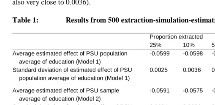
The averages of the 500 sets of estimates from Model 1 are very similar to the corresponding effect parameters used in the simulation. Most importantly from the perspective of this analysis, the average of the 500 estimates of the effect of the PSU population average is -0.0598 (see Model 1, Table 1). In comparison, -0.0600 was used in the simulation. The standard deviation of these 500 estimates is 0.0036 (and in accordance with that, each of the estimated 500 standard errors of the 500 estimates is also very close to 0.0036).

Table 1: Results from 500 extraction-simulation-estimation replications

Proportion extracted

25% 10% 5% 2.5%

Average estimated effect of PSU population average of education (Model 1)

-0.0599 -0.0598 -0.0601 -0.0601

Standard deviation of estimated effect of PSU population average of education (Model 1)

0.0025 0.0036 0.0051 0.0073

Average estimated effect of PSU sample average of education (Model 2)

-0.0591 -0.0575 -0.0555 -0.0514

Standard deviation of estimated effect of PSU sample average of education (Model 2)

0.0024 0.0036 0.0051 0.0074

Standard deviation of difference between PSU population and sample average of education

0.33 0.57 0.82 1.16

Percent difference between estimate from Model 1 and Model 2

1.3 % 3.8 % 7.6 % 14.5 %

There is a certain difference between the PSU sample average uav* calculated after

the 10% extraction and the PSU population average uav. The average of this difference

across all PSUs is approximately 0, of course, but the standard deviation of the difference across all PSUs and all 500 replications is 0.57. (In other words, the sample average is at least 0.6 years too low or too high compared to the population average in about 1/3 of the PSUs.) Because of this measurement error, the estimated effect of the sample education is not quite equal to -0.06 according to Model 2. The average across the 500 estimates is instead -0.0575, with a standard error of 0.0036. In other words, the bias is 3.8 % ((0.0598-0.0575)/0.0598 = 0.038).

(13)

procedure in principle. Fortunately, an effect that is only 5% weaker is estimated in that case: -0.0547 according to Model 2 (not shown in tables).

Let us now compare these results with those found when extractions of 25%, 5% and 2.5% are made instead (Table 1). With a 25% extraction, the standard deviation of the measurement error in the PSU-level education average is 0.33. The average of the estimated effects of the population average is -0.0599, with a standard deviation of 0.0025, while the effect of the sample average is -0.0591, with a standard deviation of 0.0024. With a 5% extraction, the measurement error is larger, of course, and the average estimate from Model 2 is -0.0555, with a standard deviation of 0.0051. With a 2.5% extraction, the corresponding figures are -0.0514 and 0.0074, respectively. Thus, a 15% bias is introduced.

The size of the population in each PSU differs widely. An average of 1000, including 250 women of reproductive age, has been assumed here. However, it is more likely to be smaller than this, than to be larger. If we assume a size of 500, and therefore also establish a population that is 5 times as large as the DHS sample instead of 10 times as large, and make a 20% rather than 10% extraction, the bias turns out to be 3.4% instead of 3.8% (see further discussion of cluster and population sizes below).

The next step is to try other model assumptions. First, the event is “made” less or more frequent, by changing the constant term in the simulation. Second, weaker and stronger education effects are tried. Neither of these changes have appreciable impact on the size of the bias, as measured in % (not shown in tables).

(14)

Table 2: Results of 5000 extraction-simulation-estimation replications, performed on a random 1/10 of the PSUs

25% 10% 5% 2.5%

-0.0601 -0.0601 -0.0601 -0.608

0.0075 0.0120 0.0170 0.0238

-0.0593 -0.0576 -0.0552 -0.0518

0.0075 0.0119 0.0168 0.0242

0.33 0.58 0.84 1.19

1.3 % 4.2 % 8.2 % 14.8 %

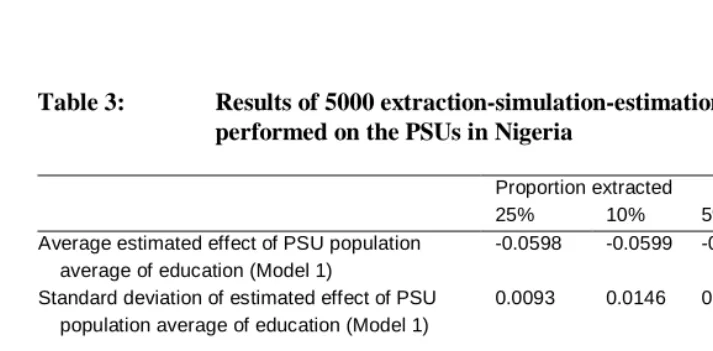
Table 3: Results of 5000 extraction-simulation-estimation replications, performed on the PSUs in Nigeria

25% 10% 5% 2.5%

-0.0598 -0.0599 -0.0602 -0.603

0.0093 0.0146 0.0208 0.0299

-0.0592 -0.0582 -0.0567 -0.0536

0.0094 0.0148 0.0213 0.0312

0.34 0.59 0.86 1.22

(15)

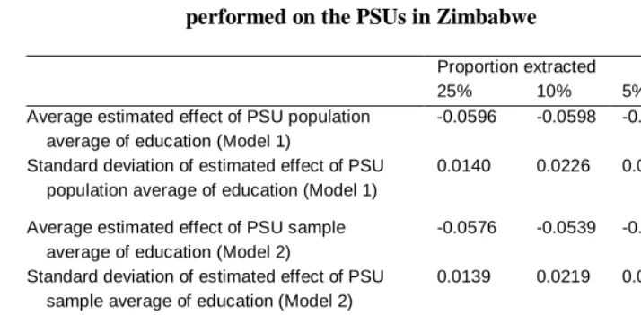
Table 4: Results of 5000 extraction-simulation-estimation replications, performed on the PSUs in Zimbabwe

25% 10% 5% 2.5%

-0.0596 -0.0598 -0.0596 -0.590

0.0140 0.0226 0.0320 0.0451

-0.0576 -0.0539 -0.0485 -0.0406

0.0139 0.0219 0.0301 0.0410

0.34 0.59 0.85 1.21

3.4 % 9.9 % 18.6 % 31.2 %

(16)

Zimbabwe has the smallest one (0.234).7 (The difference in the ICC between Nigeria and Zimbabwe is a result of a much larger between-PSU variance in education in the former country, combined with an only marginally larger within-PSU variance.) In Kenya, the ICC in education is somewhat higher than it is in Zimbabwe, but the bias is nevertheless somewhat larger (13.8%), probably as a result of the smaller size of the clusters (15).

To check more formally whether there is a relationship between the bias on the one hand and the ICC and the absolute cluster size on the other (still given that the clusters are 10% of the PSU populations), linear regression models are estimated from the results for the 16 countries (i.e. the bias, ICC and average cluster size for one country constitute one observation). Not knowing what functional form would be most appropriate, it is experimented with various logarithmic and logistic transformations. In all of these models, a higher ICC and a higher average cluster size are found to lower the bias.

The implication of these results for the 16 African countries is that researchers may safely estimate such simple multilevel hazard models – from any kind of data - as long as the ICC of the independent variable in focus (not necessarily education) is in the same range as here (at least about 0.2), and clusters are at least as large, in absolute and relative terms. However, what would happen if one moves away from this situation, towards, for example, much lower ICC values? According to predictions from the various regression models estimated from the results for the 16 countries, the bias may exceed 30-40% when the ICC dips below 0.100 (cluster sizes assumed fixed at the average for the African data). The models may not perform well outside the range of the data for which they are estimated, though. To check further into this issue, let us consider the approximately 1/10 of the PSUs that have the largest within-PSU variance in education - the precise selection criterion being a standard deviation larger than 3.5. Using this sub-population, the measurement errors are larger than those obtained in the other simulation experiments (compare Table 5 with Tables 1-4). There is also less

variation between PSUs in this sub-population8, so the ICC is only 0.0648. Of course,

this is a weird selection from the African DHS samples, not reflecting any particular real population. However, that should be of little concern. The key issue is that, in some data, there may be variables that are relevant to include in a model and for which the

7

It may be noted that these ICC values are calculated from the Nigerian and Zimbabwean parts of the pooled population built up from all DHS surveys. Because the construction of this population is based on a model estimated jointly from all DHS samples, the ICC values calculated from the DHS surveys are somewhat different (0.530 in the Nigerian DHS and 0.270 in the Zimbabwean DHS). For all 16 countries pooled, the intra-class correlation is, of course, the same in the DHS surveys as in the population (0.524 and 0.528, respectively).

8

(17)

ICC is as low as this. Anyway, according to the simulations based on this sub-population, the bias in the effect of average education is as large as 19 % with a 25% extraction, 42% with the “standard” 10% extraction, and 60 % with a 5% extraction.

Table 5: Results of 5000 extraction-simulation-estimation replications, performed on PSUs where the standard deviation of individual education is greater than 3.5 (about 1/10 of the PSU).

25% 10% 5% 2.5%

-0.0600 -0.0607 -0.0607 -0.0602

0.0168 0.0264 0.0378 0.0545

-0.0485 -0.0352 -0.0246 -0.0155

0.151 0.0208 0.0252 0.0303

0.46 0.79 1.15 1.62

19.2 % 42.0 % 59.5 % 74.3 %

In two other peculiar sub-populations that are considered, with ICC values of about 0.10 and 0.15 and cluster sizes around 24, the biases resulting from 10% extractions are 28% and 17%, respectively. In a third sub-population where the ICC is also almost 0.1, but the cluster size is 36, the bias is 22% (as opposed to 28% with a cluster size of 24). Finally, the bias is as small as 2% in a sub-population where the ICC is about 0.6 and the cluster size is 46. These results lend further support to the idea that the bias increases as ICC or cluster size are reduced.

(18)

and 50) outside the range of the country averages in the African data, produce biases of 14.9% and 1.8%, respectively. The biases are shown in Table 6, in the row labelled 10%.

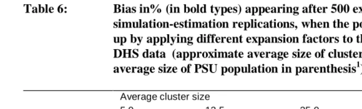
To summarize, the bias increases with decreasing absolute cluster size, given their relative size. Conversely, given the size of the PSU population, the bias increases with decreasing relative size (% extracted). The latter appears clearly in all the tables 1-5. What remains to be described is how the bias is influenced by the relative size of the clusters, given their absolute size. This is now done by experimenting not only with a variety of (integer) expansion factors, as above, but also the proportion extracted. Some examples based on the complete African data set (i.e. the data on which Table 1 is based) are given in Table 6. If we compare within columns, i.e. for a fixed absolute cluster size, we see that there is little impact of the extraction factor above a certain level. However, the bias is bound to approach 0 as the sample gets more and more equal to the population (i.e. approaching 100% extraction). An important conclusion from Table 6 is that, with an absolute cluster size above 12, the bias is always less than 8%, regardless of the size of the clusters and the corresponding PSU populations. Should a bias of 20% be deemed acceptable, one might even work with clusters including only 5 respondents.

Table 6: Bias in% (in bold types) appearing after 500 extraction- simulation-estimation replications, when the population is built up by applying different expansion factors to the entire pooled DHS data (approximate average size of cluster / approximate average size of PSU population in parenthesis1)

Average cluster size

5.0 12.5 25.0 50.0

100% 2 0 0 0 0

50.0% 4.0 (12.5 / 25) 2.0 (25 / 50) 1.0 (50 / 100)

20.0% 13.4 (5 / 25)

10.0% 14.9 (5 / 50) 6.9 (12.5 / 125) 3.8 (25 / 250) 3 1.8 (50/ 500)

2.5% 17.5 (5 / 200) 7.8 (12.5 / 500) 4.2 (25 / 1000) 2.1 (50 / 2000)

0.625% 17.6 (5 / 800) 7.8 (12.5 / 2000)

1

The approximate average size of the PSU population is defined as 25 times the expansion factor, and the approximate average size of the cluster is defined as 25 times the expansion factor multiplied by the proportion extracted.

2

(19)

The picture looks different when a similar set of simulation experiments are performed on data for Zimbabwe, where the ICC is only about 0.2. In this case, a bias less than 10% can only be achieved with clusters larger than about 25 or very large extractions (Table 7). Finally, let us turn to the peculiar sub-sample consisting of clusters where the standard deviation of education is higher than 3.5. With these data, a bias of 10% cannot even be achieved with 50% extractions as long as the clusters are smaller than 50 (Table 8).

Table 7: Bias in % (in bold types) appearing after 5000 extraction- simulation-estimation replications, when the population is built up by applying different expansion factors to the Zimbabwean DHS data (approximate average size of cluster / approximate average size of PSU population in parenthesis1)

5.0 12.5 25.0 50.0

100% 2 0 0 0 0

50.0% 8.8 (12.5 / 25) 5.5 (25 / 50) 2.8 (50 / 100)

20.0% 28.1 (5 / 25)

10.0% 33.3 (5 / 50) 16.9 (12.5 / 125) 9.9 (25 / 250) 33 5.2 (50 / 500)

2.5% 35.2 (5 / 200) 20.0 (12.5 / 500) 11.1 (25 / 1000) 5.9 (50 / 2000)

1_{The approximate average size of the PSU population is defined as 25 times the expansion factor, and the approximate average} size of the cluster is defined as 25 times the expansion factor multiplied by the proportion extracted.

(20)

Table 8: Bias in % (in bold types) appearing after 5000 extraction- simulation-estimation replications, when the population is built up by applying different expansion factors to the clusters in the pooled DHS data for which the standard deviation of individual education is greater than 3.5 (approximate average size of cluster/ approximate average size of PSU population in parenthesis1)

5.0 12.5 25.0 50.0

100% 2 0 0 0 0

50.0% 25.1 (12.5 / 25) 16.8 (25 / 50) 12.3 (50 / 100)

20.0% 55.4 (5 / 25)

10.0% 62.5 (5 / 50) 51.4 (12.5 / 125) 42.0 (25 / 250) 3 31.6 (50 / 500)

2.5% 75.2 (5 / 200) 68.2 (12.5 / 500) 54.6 (25 / 1000) 39.7 (50 / 2000)

1_{The approximate average size of the PSU population is defined as 25 times the expansion factor, and the approximate average} size of the cluster is defined as 25 times the expansion factor multiplied by the proportion extracted.

2_{Not calculated. The bias is 0 by necessity.} 3_{The same as in Table 5}

4. Conclusion

The bias introduced by using cluster averages based on about 25 women as proxies for the PSU population averages is very small – only about 4% - when all the about 5000 PSUs in 16 DHS surveys in sub-Saharan Africa are included in a first-birth model. Moreover, one may well use a small random sample of these PSUs, or use PSUs from only one country. The bias in these situations is always below 14%. (But the standard errors of the estimates become larger, of course, when a smaller material is used.)

(21)

increases as this ratio is reduced . The bias also increases with decreasing absolute or relative size of the clusters.

Apparently, researchers need not worry much about the bias, which would not be higher than about 10%, if they use data where the clusters include 25 or more persons and the relevant ICC value is above 0.2. Of course, if the clusters are much larger than that, or the ICC values are much higher, the bias will be smaller. On the other hand, if the cluster sizes are as here and the ICC is substantially below 0.2 - because of relatively large variation within and/or little variation between communities - the bias may become unacceptable. It would help with more persons in each cluster, of course, but a quite large size may be needed. For example, in the peculiar population where the ICC in education is only 0.0648, not even clusters of 50 persons drawn from PSU populations of 100 give a bias below 10%. Conversely, if the ICC is above 0.2, as in the African data, but the cluster sizes are much smaller than the average of 25 for these countries, the bias may also be large. The most extreme example among the 16 countries is Kenya, where the clusters include only 15 persons on average and the bias is 14% (while it is less than 10% in all other countries). With clusters even smaller than that, the bias may soon become unacceptable.

The bias has not been calculated for all possible combinations of ICC and cluster size, but the few numbers given should provide some guidance. For researchers who estimate more complex types of multilevel models, or who use data with a structure outside the range of the illustrations in this investigation, it might be helpful to perform simulation experiments similar to those reported here.

5. Acknowledgements

(22)

References

Angeles, G., Guilkey, D.K., and Mroz, T.A. (1998). “Purposive program placement and the estimation of family planning effects in Tanzania.” Journal of the

American Statistical Association, 93: 884-899.

DeRose, L. and Kravdal, Ø. (2006). ”Educational reversals and first-birth timing in sub-Saharan Africa: A dynamic multilevel perspective.” Forthcoming in

Demography.

Goldstein, H. (1995). Multilevel Statistical Models, second ed. Arnold: London

Greene, W.H. (2003). Econometric analysis, 5th edition. Prentice Hall: Upper Saddle

River (NJ).

Kravdal, Ø. (2002). “Education and fertility in sub-Saharan Africa: Individual and community effects.” Demography, 39: 233-250.

Macro International Inc. (1996). Sampling Manual. DHS-III Basic Documentation. No. 6. Calverton, Maryland.

Montgomery, M.R. and Casterline, J.B. (1996). “Social learning, social influence and new models of fertility.” Population and Development Review, 22 suppl: 151-175.

Montgomery, M. and Hewett, P.C. (2005). "Urban poverty and health in developing countries: Household and neighborhood effects". Demography, 42: 397-425