Meta State Generalized Hidden Markov Model for Eukaryotic Gene Structure Identification

(1)

University of New Orleans University of New Orleans

ScholarWorks@UNO

University of New Orleans Theses and

Dissertations Dissertations and Theses

12-20-2009

Meta State Generalized Hidden Markov Model for Eukaryotic Gene

Structure Identification

Carl Baribault

University of New Orleans

Follow this and additional works at: https://scholarworks.uno.edu/td

Recommended Citation Recommended Citation

Baribault, Carl, "Meta State Generalized Hidden Markov Model for Eukaryotic Gene Structure Identification" (2009). University of New Orleans Theses and Dissertations. 1098.

https://scholarworks.uno.edu/td/1098

This Dissertation is protected by copyright and/or related rights. It has been brought to you by ScholarWorks@UNO with permission from the rights-holder(s). You are free to use this Dissertation in any way that is permitted by the copyright and related rights legislation that applies to your use. For other uses you need to obtain permission from the rights-holder(s) directly, unless additional rights are indicated by a Creative Commons license in the record and/ or on the work itself.

(2)

Meta State Generalized Hidden Markov Model for Eukaryotic Gene Structure Identification

A Dissertation

Submitted to the Graduate Faculty of the University of New Orleans in partial fulfillment of the requirements for the degree of

Doctor of Philosophy in

Engineering and Applied Science Computer Science/Bioinformatics

by

Carl Edward Baribault

B.S. Loyola University, New Orleans, LA, 1978 M.S. University of North Carolina at Chapel Hill, 1981

M.A. University of Texas at Austin, 1986

(3)

Dedication

(4)

Acknowledgment

Funding for this effort was derived from grants from NIH, NSF, LA Board of Regents, and NASA.

To the members of my committee, thanks in general for their perseverance and critical input. In particular, thanks to Dr. Huimin Chen for his guidance in formulating the factorizations of the HOHMM in this effort. Thanks to my advisor, Dr. Steven Winters-Hilt for providing the initial versions of the theory and code for the HOHMM and for his support and guidance

throughout this effort. In my humble opinion, Dr. Winters-Hilt with his outstanding background and cross-disciplinary knowledge is a credit to the institution of the University of New Orleans as well as the Louisiana State University system.

To my research colleagues, A. Murat Eren, Brian Roux, Zuliang Jiang, and Alex Lu, thanks for their collaboration and provision of supporting material for this thesis. Thanks also, to all other members of Dr. Winters-Hilt‟s bioinformatics research team for all their cooperation.

To members of the UNO Department of Computer Science thanks for their supporting roles. In particular, thanks to the chairman, Dr. Mahdi Abdelguerfi, for his generous support. Thanks to the secretary, Ms. Jeanne Boudreaux, for all of her efforts and cooperation in

processing payroll related forms, etc. Thanks also to the system administrator and colleague, Mr. Fareed Qaddoura, for his advice and help in keeping the various department servers in working order.

Finally, thanks to the members of my extended family for their various supporting roles – as well as their prayerful requests for my progress. Thanks to my wife, Sandra, for all her

(5)

List of Figures

Figure 1 Factor graph for traditional, 1st order HMM. ... 9

Figure 2 Stepwise association (or clique) of observations and hidden states in HOHMM ... 12

Figure 3 Comparison of theoretical relative time complexity – linear scale ... 26

Figure 4 Comparison of theoretical relative time complexity – log scale ... 27

Figure 5 A sample of HOHMM test times for test data length 1Mb ... 43

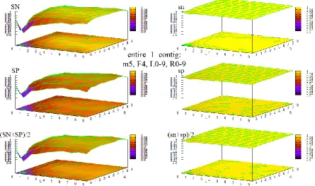
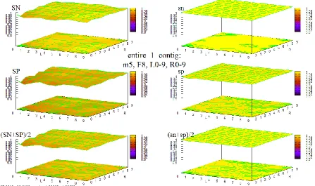
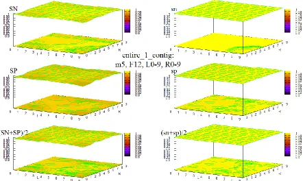
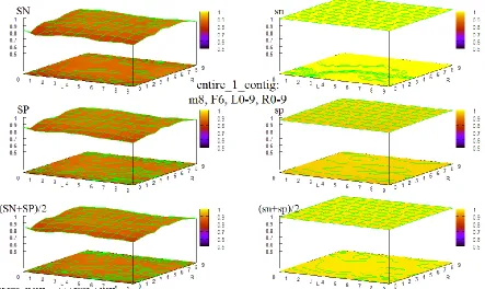
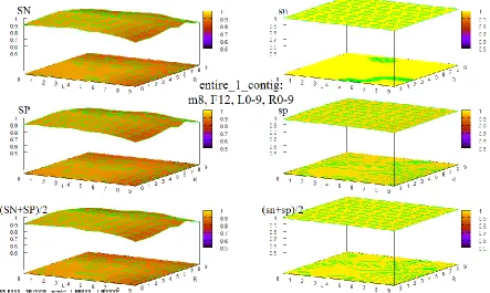
Figure 6 Maximum full exon HOHMM performance for data entire_1_contig... 51

Figure 7 Maximum base level HOHMM performance for data entire_1_contig ... 51

Figure 8 Maximum full exon HOHMM performance for data ALLSEQ ... 57

Figure 9 Maximum base level HOHMM performance for data ALLSEQ ... 57

Figure 10 Full exon level accuracy for C. elegans 5-fold cross-validation (F view) ... 63

Figure 11 (Nucleotide) Base level accuracy for C. elegans 5-fold cross-validation (F view) ... 63

Figure 12 Full exon level accuracy for C. elegans 5-fold cross-validation (M view)... 64

Figure 13 (Nucleotide) Base level accuracy for C. elegans 5-fold cross-validation (M view) ... 64

Figure 14 Summary of relative entropy, H(P(eij, M, i), P(xx, M,i)), for reduced C.E., I-V with log scaling. (Graphs are arranged vertically according to base Markov order, M, and horizontally according to classes of transition dimer, je0/e2j(left), ei(middle), and ie(right).) ... 67

Figure 15 Average accuracy of Viterbi decoding using 1-step approximation of 1k-step generating duration model... 73

Figure 16 Standard deviation of accuracy of Viterbi decoding using 1-step approximation of 1k-step generating duration model ... 73

Figure 21 Average accuracy of Viterbi decoding using same 1k-step decoding duration model as 1k-step generating duration model ... 76

Figure 22 Standard deviation of accuracy of Viterbi decoding using same 1k-step decoding duration model as 1k-step generating duration model ... 76

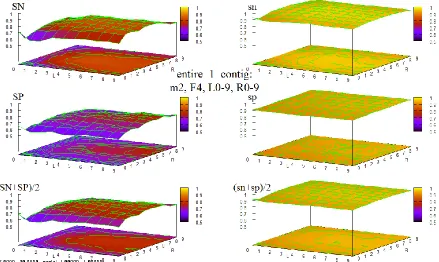
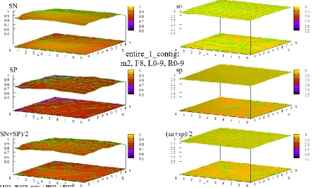
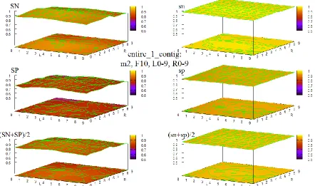
Figure 23 HOHMM performance for data entire_1_contig using m=0, F=4, L=0-9,R=0-9 ... 89

(10)

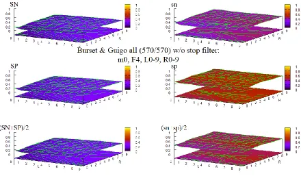
Figure 43 HOHMM performance for B & G data using m=0, F=4, L=0-9,R=0-9 ... 100

Figure 49 HOHMM performance for B & G data using m=2 , F=6, L=0-9,R=0-9 ... 103

Figure 63 HOHMM performance using C.E. I-V (alt. splicing deleted) m=0, F=2, L=0-9,R=0-9 ... 111

(11)

(12)

Figure 95 HOHMM performance using C.E. I-V (alt. splicing deleted) m=8, F=6, L=0-9,R=0-9 ... 127 Figure 96 HOHMM performance using C.E. I-V (alt. splicing deleted) m=8, F=8, L=0-9,R=0-9 ... 127 Figure 97 HOHMM performance using C.E. I-V (alt. splicing deleted) m=8, F=10, L=0-9,R=0-9 ... 128 Figure 98 HOHMM performance using C.E. I-V (alt. splicing deleted) m=8, F=12, L=0-9,R=0-9 ... 128 Figure 99 HOHMM performance using C.E. I-V (alt. splicing deleted) m=8, F=14, L=0-9,R=0-9 ... 129 Figure 100 HOHMM performance using C.E. I-V (alt. splicing deleted) m=8, F=16, L=0-9,R=0-9 ... 12L=0-9,R=0-9 Figure 101 HOHMM performance using C.E. I-V (alt. splicing deleted) m=8, F=18, L=0-9,R=0-9 ... 130 Figure 102 HOHMM performance using C.E. I-V (alt. splicing deleted) m=8, F=20, L=0-9,R=0-9 ... 130 Figure 103 Relative entropy, H(P(je0, M, i), P(jj, M)), for reduced C.E., I-V with log scaling. ... 132 Figure 104 Relative entropy, H(P(je0, M, i), P(jj, M)), for reduced C.E., I-V with max scaling. ... 132 Figure 105 Relative entropy, H(P(e0i0, M, i), P(ee, M,i)), for reduced C.E., I-V with log

scaling. ... 133 Figure 106 Relative entropy, H(P(e0i0, M, i), P(ee, M,i)), for reduced C.E., I-V with max scaling. ... 133 Figure 107 Relative entropy, H(P(e1i1, M, i), P(ee, M,i)), for reduced C.E., I-V with log

scaling. ... 134 Figure 108 Relative entropy, H(P(e1i1, M, i), P(ee, M,i)), for reduced C.E., I-V with max scaling. ... 134 Figure 109 Relative entropy, H(P(e2i2, M, i), P(ee, M,i)), for reduced C.E., I-V with log

(13)

Figure 117 Relative entropy, H(P(e2j, M, i), P(ee, M,i)), for reduced C.E., I-V with log scaling.

... 139

Figure 118 Relative entropy, H(P(e2j, M, i), P(ee, M,i)), for reduced C.E., I-V with max scaling. ... 139

Figure 119 SVM: Hyper plane separability with a Margin (thickness). Support vectors consist of both the blue and red points occurring on the blue and red margin surfaces, respectively. Unlike HMM-based classification, the SVM-classification provides built-inconfidence levels as part of the classification output. ... 140

Figure 120 Flowchart for Main Sequence on Client – Includes 1)Training and 2)Testing... 142

Figure 121 Flowchart for Client Task List Processing - Applies to 1)Training or 2)Testing... 143

Figure 122 Flowchart for Client Task - Applies to 1)Training or 2)Testing ... 144

Figure 123 Flowchart for Server Training Task ... 145

Figure 124 Flowchart for Server Training Task, cont. ... 146

Figure 125 Flowchart for Server Testing Task ... 147

(14)

Abstract

Using a generalized-clique hidden Markov model (HMM) as the starting point for a eukaryotic gene finder, the objective here is to strengthen the signal information at the transitions between coding and non-coding (c/nc) regions. This is done by enlarging the primitive hidden states associated with individual base labeling (as exon, intron, or junk) to substrings of primitive hidden states or footprint states. Moreover, the allowed footprint transitions are restricted to

those that include either one c/nc transition or none at all. (This effectively imposes a minimum length on exons and the other regions.) These footprint states allow the c/nc transitions to be seen sooner and have their contributions to the gene-structure identification weighted more heavily – yet contributing as such with a natural weighting determined by the HMM model itself according to the training data – rather than via introducing an artificial gain-parameter tuning on major transitions. The selection of the generalized HMM model is interpolated to highest Markov order on emission probabilities, and to highest Markov order (subsequence length) on the footprint states. The former is accomplished via simple count cutoff rules, the latter via an identification of anomalous base statistics near the major transitions using Shannon entropy. Preliminary

indications, from applications to the C. elegans genome, are that the sensitivity/specificity

(SN/SP) result for both the individual state and full exon predictions are greatly enhanced using the generalized-clique HMM when compared to the standard HMM. Here the standard HMM is represented by the choice of the smallest size of footprint state in the generalized-clique HMM. Even with these improvements, we observe that both extremely long and short exon and intron segments would go undetected without an explicit model of the duration of state.

The key contributions of this effort are the full derivation and experimental confirmation of a rudimentary, yet powerful and competitive gene finding method based on a higher order hidden Markov model. With suitable extensions, this method is expected to provide superior gene finding capability – not only in the context of pre-conditioned data sets as in the evaluations cited but also in the wider context of less preconditioned and/or raw genomic data.

(15)

1 Introduction

1.1 Background

This work is largely a study in the extension of the traditional, 1st order hidden Markov model (HMM) to be used in the analysis of genomic signals, but some mention is also made of significant supporting roles played by Support Vector Machines (SVM‟s). The complementary capabilities of HMM feature extraction and SVM classification can be combined to produce highly effective approaches to signal processing in both genomic and cheminformatic settings as well.

The use of 1st order HMM in genomic signal processing is expected to have limited results in light of observed fluctuations of not only 1st order relative entropy but also that for higher orders over extended regions surrounding coding/non-coding (c/nc) boundaries in DNA sequence data. In general, attempts to employ higher order HMM‟s (HOHMM) can result in an exponential explosion of states and hence run-time complexity, where each HOHMM state is a fixed-length, but otherwise less restricted (though not entirely arbitrary) concatenation of primitive exon (e), intron (i), and junk (j) states.

This thesis presents an HOHMM using a minimum-length assumption, where coding and

non-coding segments are assumed to be bounded in length from below, with the reasonable penalty of an additional, post-processing step in order to handle the shorter segments excluded from the ensuing prediction as a result. The advantage of this minimum-length assumption is a scalable HOHMM with linear complexity in the length of the extended states or footprint states.

1.2 Related Work

Computational gene finding dates back to the mid 1980‟s if not further [1]. New gene

finding programs arose up until about the year 2000. Afterward came a period of publication of summaries of gene finding programs until 2003. Since that time up until the present, the

available literature is generally in the area of sensors for detecting specific sites or features, such c/nc transitions, gene starts, etc.

One approach to gene finding used in homology-based programs generally attempts to

identify new genes by characterizing the sequence alignments among known genes, such as in [2]. Another more recent effort discussed in [3], combines homology information with other ab initio information or intrinsic, statistical properties of the DNA sequence alone. In general, the

main drawback of homology-based approaches is that they appear incapable of finding new genes. See, for example, in [4], where a study is cited in [5], in which only 50% of the proteins

encoded in human chromosome 22 were found to be similar to previously known proteins. As mentioned above, much of the effort in recent years has been expended in the development of specific sensors, such as those listed in Table 1 below. In general, these programs require (and in some cases provide) an external interface for incorporation into a comprehensive, structural gene identification system, for example, see 5.2 Future Work, page

(16)

Table 1 Programs for genetic feature sensors among the related work

Program Name

Targeted Feature Description Reference

MetaTISA Transcription initiation sites (TIS)

Classification via phylogenetic clustering of genomic sequence data

[6]

WordSpy Transcription factor binding motifs (TFBM)

Dictionary and grammar for sequence motifs + EST similarity

[7]

MZEF Internal exons in human genes Classification of genomic sequence features via quadratic discriminant analysis (QDA)

[8]

SpliceMachine splice sites SVM classification of splice site

and exon content features

[9]

FirstEF promoters and first exons Classification of features in promoter and first donor splice sites via QDA

[10]

DNAFSMiner TIS in vertebrate DNA/mRNA/cDNA, polyadenylation in human DNA

SVM classification of entropic/Markov features of target sites

[11]

Splice sites SVM classification with

weighted degree kernel

[12], [13]

PEAKS Regulatory motifs in DNA Frequency of motifs near target feature sites

[14]

Splice sites, translation start sites (TSS‟s), TIS

Neural network classification of higher order Markov

dependencies at target sites

[15]

Gene 3´ ends (stops) Classification via positional clustering of polyadenylation sites of known transcripts

[16]

1.3 Organization of This Thesis

In 2 Structural Gene Prediction via HOHMM, as the main body of work in this effort,

we develop a higher order HMM (HOHMM) in order to predict the genetic structure of lower order eukaryotic genomes. We observe that the scalability of the computation is realized by allowing only those hidden states in a relatively small but reasonably representative subset of the Cartesian product, ΛF+1_{, where}_Λ_{is the alphabet of primitive hidden states, and where the subset} grows linearly in F, the footprint state size in consecutive (but overlapping by one primitive)

(17)

In 3 HOHMM Implementation and Results, page 44, first there is an overview of the

implementation including the organization at the top level of the client-server architecture

common to both the training and testing facilities. Following that are the results of testing with 3 data sets, entire_1_contig of C. elegans, the benchmark data set ALLSEQ assembled by Burset

& Guigo in [17], and data-reduced versions of Chromosomes I-V of C. elegans [18]. In the first

two cases of the entire_1_contig and ALLSEQ data sets, we use the same data set for both training and testing in order to exhibit a simple, brute force search for optimum values of the HOHMM parameters. The 3rd data set has been data-reduced in order to remove alternative splicings. Using that data set we show the results of testing with 5-fold cross-validation. We also include graphs of relative entropy and a discussion of its usefulness for the various types of c/nc transitions identified in the annotation data for this last data set, where the entropy values have been computed in a window centered on the respective transition sites.

In 4Other HMM Applications, page 68,first we mention several other applications

based on iterative HOHMM processing. Then we include a treatment taken largely from [19] on

a form of duration modeling to the HMM (HMMwD) where the form is exact in the 2-state case in that there is no ambiguity of the destination state upon exit of a given state duration. This work has served to motivate the development of an exact, implicit HMMwD [20]. Either the

approximate or the exact formulation can be used to extend the HOHMM to include duration submodels for introns and exons in order to improve splice site recognition. Here the future intent would be enhanced recognition of both unusually short as well as unusually long instances of both exons and introns. We also include the results of successful, preliminary trials of the HMMwD on synthetic data [19].

Also in 4.3 Controlled Acquisition via SVM, page 77, and 4.4 Pattern Recognition Informed Feedback via LabWindows Automation, page 78, we briefly describe ongoing

efforts in measurements involving real time molecular capture and acquisition and control of pico-amp (pA) ion current signals induced by that capture at the site of a highly narrow protein channel called a nanopore. Also, with material taken largely from [21] we present the first

functional prototype of a nanopore signal acquisition system using SVM-based identification and control of the molecular species captured at the nanopore channel site. Continuation of this work discussed in [22].

In 5 Discussion and Future Work, page 79, we discuss the results of the HOHMM

referring also to the results in the two evaluations cited. We also discuss some issues associated with the testing methodology in the evaluations cited and the impact on the programs evaluated. Finally, we provide perspective on the HOHMM and its greater usefulness in a wider context of gene finding.

6 is Bibliography, page 83, and in 7 Appendix, page 88, there are detailed results of

testing in the form of extended sequences of (combined contour and 3D surface) graphs of accuracy of the HOHMM for all values tested of the 4 main parameters in the model, M, F, L, and R. These extended sequences of graphs provide a compelling demonstration of the stability of the HOHMM with respect to the choice of those 4 parameter values for all such values tested. There is also in 7 an extended, fully connected, 7-page flowchart depicting the function and

(18)

client-server infrastructure is implemented in Perl. The C-based portion of the testing code, the Viterbi engine, is contained entirely within the server side.

1.4 Contributions

It should be noted that the original HOHMM derivation and code implementation (in Perl and C) were done in their initial form by my Ph.D. thesis advisor, Dr. Winters-Hilt [23]. When

first presented to me, however, he indicated that there appeared to be an insidious run-time bug in the code implementation and that, although the implementation was 95% complete and

operated with some predictive power (~70% accuracy), it was hopelessly flawed. My task, thus, began with learning how to do run-time debugging of a complex higher order HMM. I was warned that HMM implementation errors that only show at run-time are very complicated to isolate, and this was indeed the case, as born out by my thorough review and rederivation of the theory outlined in [24]. As a direct result of my review, the bug was identified and found to be

due to a minor, but critically significant approximation error in the theoretical description itself and that this error had previously been faithfully represented in the code. Upon repairing the code with the correct underlying theory, the predictive power on the test data improved to 99% accuracy on the base-by-base prediction of coding state (exon) versus non-coding state (intron or junk) using the diagnostic data set (or training contig), entire_1_contig of C. elegans. (See 3.4.2

Summary of Results for Entire_1_contig of

C. elegans

, page 50.)

Moreover, the correct factorization of total probability for the HOHMM is presented in two different forms, each with accompanying sample calculation. As suggested above, the first form of factorization had already been outlined by my advisor, Dr. Winters-Hilt in [24]. The

final, corrected form is presented in 2.5 Factorization 1 of Total Probability, page 27, and

clearly indicates the proper formulation for future extension via SVM-based discriminator as demonstrated to some extent in [25]. The 2nd form of factorization is also a contribution in this

effort, and also admits formal substitution of an SVM-based discriminator. Though no testing was performed with this alternate form in this effort, this form was introduced to also link most closely with standard autoregressive HMM descriptions. (See, for example, [26].)

Another contribution in this effort is included in 2.10Alternate Proof of Linear Upper Bound on Footprint States and Transitions, page 39. This provides a more compact and

concise argument for demonstrating the linear limit of growth of the HOHMM‟s complexity with respect to footprint state size – without the need for the full enumeration and precise counting of footprint states as shown in 2.4 Linear Growth in State/Transition Space, page 14.

Last but not least in terms of man-hours among the contributions in this effort is the additional software architectural features (design) and coding effort (implementation) for the training and testing phases of the HOHMM, including among others:

1) a Perl-syntax based, hence fully programmable, user configuration input file for defining:

a. units of work or tasks for both training and testing of the HOHMM, and

b. full specification of the distribution and multi-threaded execution (via Perl threads) of those tasks among both task-specific and/or generic sets of processors available via public key authentication

2) a Perl based, reusable, client/server, multi-task, distributed processing architecture – reused for performing both training and testing tasks

3) a well-defined, hence extendable interface for task execution in multiple job scheduling contexts, including the currently implemented interfaces for:

(19)

b. LoadLeveler job scheduling as implemented for the IBM/AIX OS on the IBM Power5 cluster [28].

(20)

2 Structural Gene Prediction via HOHMM

2.1 (Eukaryotic) Genomic Data

Once it is fully annotated, genomic data can be unambiguously represented by strings formed from the 4 letters a, c, g, and t denoting the DNA nucleotide bases adenine, cytosine, guanine, and thymine, respectively. Genes are units of genomic data which encode specific sequences of amino acids to form proteins. The process of annotating consists of designating

specific segments of the data as coding and non-coding (c/nc) segments. (The uppercase letters A, C, G, and T are often used to designate coding segments as distinct from the lower-cased, non-coding segments in the data.) In eukaryotes, genes consist of coding segments or exons

which are delimited internally by special, intragenic, non-coding segments or introns. The intergenic,non-coding regions of bases outside the genes are generically referred to as junk.

The process of removing the intermediate introns and reconnecting (possibly variable subsets of) the resulting exons end-to-end is referred to as splicing. Perhaps the most important

role of introns is to provide a mechanism for the formation of alternative combinations and/or subsets of the exons contained in a given gene in order to form alternative proteins also used by the organism in question. These alternative combinations are referred to as alternative splicings. 2.1.1 Framing

Exons have a 3-base encoding as directly revealed in a mutual information analysis of gapped base interpolations as shown in [23]. The 3-base encoding elements are called codons,

and the partitioning of the exons into 3-base subsequences is known as the codon framing. Thus

in order to both precisely and concisely encode a protein, the gene‟s cumulative exon string length must be a multiple of 3 bases. The term reading frame is used to denote one of the 3

possible positions – 0, 1, or 2 by our convention – relative to the start of a codon. Moreover, in general introns may interrupt genes at any point along the coding extent. In other words, introns can split the codon framing either at a codon boundary or one of two positions internal to a codon.

Although there is no notion of framing per se among introns, for convenience we associate framing with the intron, as indicated in the example below, as a tracking device in order to ensure that the frame of the immediately following exon would be predicted correctly. Finally there is neither any notion nor any use for framing among strings of junk per se. Thus we denote the primitive states of the individual bases occurring in exons, introns, and junk by members of the sets

Exon states = { e0, e1, e2 }, Intron states = { i0, i1, i2 }, and Junk state = {j}.

For example, we have 3 possible intron framings indicated in the following state strings.

(21)

2.1.2 Forward and Reverse Encoding

Encodings for proteins can be found in both directions along the DNA strand such that the two directions rarely interfere with each other. In other words, a coding segment in one encoding direction does not interfere with or overlap a coding segment in the other encoding direction. Furthermore, when comparing exons, introns, and junk segments, the estimated probabilities of occurrence of specific base sequences are substantially different, yet when comparing forward and reverse encodings the differences of such probability estimates are negligible among sequences of a given segment type – exon, intron, or junk. Hence, it would be counterproductive to simply ignore reverse encodings by relegating them to a second pass of our prediction algorithm, since that would require the interpretation of (reverse) coding segments, or exons, as junk – contradictory to that indicated by any reasonable set of estimates of the

probabilities of nucleotide occurrences.

Thus we incorporate shadow states indicating reversely encoded exons and introns into

the state model of our HOHMM, denoted by the primitives by ê and î, respectively. For example, we illustrate the 3 possible intron framings for the reverse encoding as follows:

jj...jê2ê1ê0…ê1î0î0…î0ê0…ê2ê1ê0jj…j (intron frame 0) jj...jê2ê1ê0…ê2î1î1…î1ê1…ê2ê1ê0jj…j (intron frame 1) jj...jê2ê1ê0…ê0î2î2…î2ê2…ê2ê1ê0jj…j (intron frame 2)

2.2 Limited Success with 1

st

Order HMM

We define the 1st order HMM as consisting of the following:

An observable alphabet, B A hidden state alphabet, 

(“Prior”) Probability P() for all 

(“Transition”) Probability P(2|1) for all 12 (“Emission”) Probability P(b|) for all  bB,

Given the above, there are three classes of problems [29] which the HMM can be used to

solve:

1. Evaluation - Determine the probability of occurrence of the observed sequence.

2. Learning - Determine the most likely emissions and transitions for the observed sequence.

3. Decoding (Viterbi) - Determine the most probable sequence of states emitting the observed sequence.

Here we focus only on the 3rd problem, the Viterbi decoding problem. The probability of a sequence of observables B=b0 b1… bn-1 being emitted by the sequence of hidden states =0 1…n-1 is given by

(22)

where the chain rule as been applied, resulting in the two factors known in the traditional HMM as the observation model and the state model, respectively. In the 1st order HMM, the

state model has the 1st order Markov property and the observation model is such that the current observation, bi, depends only on the current state, i. According to this, we may further factor the above probability as in the following:

P(B|) P() = (chain rule)

P(b0|) P(b1|)…P(bn-1|)

P(0)P(1|0)P(2|0, 1)…P(n-1|0...n-2)

= (1st_{order HMM states)}

P(b0|) P(b1|)…P(bn-1|)

P(0)P(1|0)P(2|1)…P(n-1|n-2)

= (1st order HMM observations)

P(b0|0) P(b1|1)…P(bn-1|n-1)

P(0)P(1|0)P(2|0, 1)…P(n-1|0...n-2)

= (regrouping)

P(0) P(b0|0) P(1|0) P(b1|1) …

P(n-1|n-2) P(bn-1|n-1)

According to [30], a factor graph is a tool frequently used in information theory to

visually specify the belief propagation algorithm by which information is propagated throughout

(23)

2 3 4 P(1|0)

P(0)

b0 b1 b2 b3 b4

1 0

P(2|1) P(3|2) P(4|3)

P(b0|0) P(b1|1) P(b2|2) P(b3|3) P(b4|4)

Figure 1 Factor graph for traditional, 1st order HMM.

The Viterbi algorithm is encoded in the factor graph using the max-product form of the belief propagation algorithm. In order to implement the Viterbi algorithm, each of the variable (square) factor nodes along the top row is to be interpreted as taking a maximum of the

probability with respect to the previous state. This results in two recursion relations, one for each of two types of values, 1) the total probability at each observation, bi and 2) the most probable state at each observation, bi . In practice, these recursively defined quantities are kept in two tables, a probabilitytable and a back pointer table, with one column in each of the two

tables for each observation, bi , and one cell or row in each column for each of the possible values of the state, i, at observation, bi .

The recursive expression for the total probability, P(bi, i) at each observation, bi , as follows:

P(bi, i) = P(bi| i) maxj [ P(i| (i-1)j ) P(bi-1,(i-1)j ) ]

where the maximum is taken over all possible values of the previous state,

(i-1)j for j = 1, … ||, and

|  | = the size of the state alphabet, .

In order to avoid having to recompute probabilities, the most probable state at each observation is computed once in dynamic programming fashion as determined by the recursive expression:

(24)

The recursion terminates with the last observation, bi , and the most probable path of states is given by

Λ* = argmax Λ P(B, Λ)

= (0*, …, 4*)

where the decoding consists of retracing through the table of back pointers starting with

4* = argmax j [P(b4, (4) j)]

With genomic data, Viterbi decoding is used to identify the coding/non-coding transition sites, such as the exon-intron and intron-exon transitions, referred to as donor and acceptor splice sites, respectively. Thus the job of gene prediction is to predict the precise locations of

such c/nc transitions within a string of genomic data. First order hidden Markov models

(HMM‟s) have been used here and elsewhere for the prediction of donor and acceptor splice sites with limited success [4]. This can be attributed to the notion that using first order statistics for

c/nc sites effectively under weights such transitions (relative to other homogeneous sites) when higher-order statistics are more appropriate in regions centered more or less on the c/nc

transitions. (Similar though weaker arguments can be made for junk-exon and exon-junk transitions as well. See, for example, [4].) This is typically revealed, for example as in 3.7 Relative Entropy of C/NC Transitions by the extent of anomalous base statistics in the

neighborhood of the transition.

2.3 Higher Order HMM (HOHMM) Specifications

As stated above, traditional 1st_{order HMM‟s assume}_{that a 1}st_{order Markov property} holds among the states and that each observable depends only on the corresponding state and not any other observable. However, the current work entails a departure from these conventions in an attempt to leverage information from the entire region of anomalous statistics in the

neighborhood of c/nc transitions (when compared to base statistics of coding or non-coding regions away from such transitions). The regions of anomalous statistics are often highly structured, having consensus sequences that strongly depart from the strong independence assumptions of the 1st order HMM. The existence of such consensus sequences suggests that we adopt an observation model that has a higher order Markov property with respect to the

observations. Furthermore, since the consensus sequences vary by the type of transition, this observational Markov order should be allowed to vary depending on the state – with higher order for non-splice sites and lower order for splice sites (where interpolation is through highest order supported by the size of the training data).

Furthermore, in the Viterbi context, for a given state dimer transition or non-transition, such as e0e1 or e0i0, respectively, we can compound the contributions of the corresponding base emissions to the correct prediction of state by using extended states. For example when encountered sequentially in the Viterbi algorithm, the following sequence of extended or

footprint states would conceivably score highly when computed in the given order at consecutive

(25)

eeeeeei,

eeeeeii,

eeeeiii,

eeeiiii,

eeiiiii, and

eiiiiii

In other words we can expect a natural boosting effect for the correct prediction at such c/nc

transitions.

In order to accommodate the above concerns, we consider the pairing of an extended observation centered on the primitive observation bi with an extended state centered on the dimer state si (see below for notation), where the observation and state extents are parameterized independently according to the following.

1) non-negative integers L and R denoting left and right maximum extents of a substring, wi, (with suitable truncation at the data boundaries, b0 and bn-1 ) associated with the primitive observation, bi , in the following way,

wi = bi-L+1, …, bi, …, bi+R ŵi = bi-L+1, …, bi, …, bi+R-1

for i = -R, …, n-R-1, where

L  0, (left extent for bases in wi)

R  0, (right extent for bases in wi)

L+R > 0. (total extent for bases in wi)

2) non-negative integers l and r denoting the left and right extents the extended (footprint) states, f, expressed usually in practice in terms of its component, overlapping dimer

states, s. Here, we show the relationships among the primitive states , dimer states s, footprint states f, and footprint transitions σ.

si = ii+1 (dimer state, length in ‟s =2) fi = si-l+1, …, si+ri-l+1, …, i, …, i+r+1 (footprint state, length in s‟s=l+r)

σi = fi-1, fi (length in s‟s= l+r+1, length in ‟s= l+r+2)  si-l, …, si+ri-l, …, i, …, i+r+1

where

l 0, (left extent of f or si-l+1, ..., si)

r  0, (right extent of f or si+1, ..., si+r)

l+r > 0. (total extent of f in s‟s)

(26)

R L

r+1 l

bases in the string wi with

M(fi-1, f, j)  0 , where

fi-1, fi = sequential footprint states,

j = the index of any member of wi in the range i-L+1  j  i+R

We note that there is no other restriction on the relative sizes of the four parameters L, R, l, and r. As in the 1st order HMM case, we assume that the ith base observation bi is aligned with the ith hidden state i. However we note in the following – as a departure from the 1st order case – that we modify the condition that bi is dependent exclusively on the hidden state i. We illustrate this pairing of specific observation strings and hidden state strings at either end and at an interior position in the processing via the diagram in Figure 2 below.

b0 … bi-L+1 … bi … bi+R … bn-1… bn+L-2… bn+L+R-2

-R-l+1…-R…-R+r+1 … i-l+1… i … i+r+1 … n+L-l-1..n+L-2..n+L+r-1

Figure 2 Stepwise association (or clique) of observations and hidden states in HOHMM

Referring to the diagram above, assuming a left-to-right traversal of the data, many choices of first and last clique are possible depending upon the desired point of onset and strength of influence from the emission probabilities in the prediction process of the Viterbi algorithm. In the case of protein product data, such choices could be critical since there is typically little, if any, buffer extent at either ends of the data for the Viterbi algorithm to recover from poorly estimated state prior probabilities. (See also 2.8 Estimates of Probabilities from Counts, page 37.)

For convenience, we have chosen the first such that the first observations, b0, is included at the leading edge. This allows the emission probabilities to exert the earliest influence on the prediction process, though the influence is weakest, since only one base, b0, is contributing at the outset. However, for the last clique, we recognize the need to predict no further than the last observation, bn-1, but we choose the trailing edge to include the last observation for convenience at the cost of making predictions for states beyond the last observation.

(27)

Table 2 Additional primitives for completion of boundary cliques

Additional Primitives Type of Primitive Boundary

-R -l+1 , …, -1 States Left

b n, …, bn+L+R-2 Observations Right

n, …, n+L+r+1 States Right

In 2.5, page 27,and 2.6, page 34, we will investigate two different factorizations of the

total probability for states and observations

P(B, Λ) = P(b0, …, bn+L+R-2 ; -R -l+1, …, n+L+r-1)

noting that both factorizations represent departures in their own varying degrees from the factorization of the traditional HMM. The first factorization departs immediately from the traditional separation between observation and state models, but the second does at least initially separate the observation and state models.

We will observe that both factorizations allow for an alternate representation such that the internal scalar-based state discriminant can be replaced with a vector-based discriminant. This would allow the substitution of a discriminant based on a Support Vector Machine (SVM) as demonstrated for splice sites in [25]. Also, we note that these alternate representations would

not introduce any significant increase in computational complexity, since the SVM-based discriminant, having been trained offline, would require the computation of a simple vector dot product.

2.3.1 Assumptions

We demonstrate in 2.4 Linear Growth in State/Transition Space below the fact that the

number of allowed transitions among footprint states is restricted to the linear growth in the size of the footprint states. First, we first list the assumptions used as well as some mostly notational conventions in 2.3.2 Conventions below.

1) The length of introns and exons are bounded below, such that the following hold: a. footprint states can contain at most one coding/non-coding (c/nc) transition b. footprint state transitions can involve at most one c/nc transition among both the

source and destination footprint states

(This is referred to as the minimum length assumption. See parameter F defined below

in Conventions.)

2) The length distributions of introns and exons are taken to be geometric by default. (See [20] and [4].)

3) We introduce support in the model for the notions of reading frame (0, 1, 2) and encoding direction (forward, reverse), thus replacing the basic exon e and intron i state primitives with the set of state primitives e0,e1,e2,i0,i1,i2,ê0,ê1,ê2,î0,î1,î2. Without such explicit support in the model for the reverse encoding, we incur undue risk of

indeterminate results [24]. For example, consider the case of a small, reverse encoded

(28)

4) We make no attempt to encode the notions of reading frame or encoding direction in the case of junk, hence designating a single primitive junk state, j.

5) The base Markov order, with maximum value specified by parameter M of the HOHMM, is allowed to vary below the maximum M as a function of both footprint state as well as the position of the observed base relative to the c/nc transition site within the footprint state.

6) We make no attempt thus far to vary the base Markov emission extent with respect to the encoding direction. For example, we use the value R to designate the right base emission extent for both the 3‟-side in the context of forward transitions as well as the 5‟-side in the context of reverse (shadow) transitions. Whereas, otherwise, we would anticipate some overall improvement in prediction accuracy of the HOHMM.

2.3.2 Conventions

1) According to Figure 2 above, a footprint state is an extended state consisting of l+r+1 primitive states. In practice, however, we use a symmetric footprint state, where l = r, and we denote the size of the footprint states for a given instance of an HOHMM by a single parameter F, where F is measured in units of consecutive, overlapping dimers. Thus, we write

F = 2l = 2r = length of footprint state in dimers.

2) In the following we will use the symbols ê, î in order to denote exon and intron primitive states for the reverse encoding direction. Yet when we refer to the

corresponding footprint states by name the primitives will be listed in 5‟-to-3‟, encoding order, such as the dimer ê0î0, and the dimer transition ê0î0 to î0î0. Thus, we have the following complete set of state primitives.

Set of state primitives = { e0,e1,e2,i0,i1,i2,ê0,ê1,ê2,î0,î1,î2,j }

3) The reading frame varies cyclically among the primitives within an exon, such as e0e1e2, whereas the reading frame of an intron is fixed over the entire segment of intron

primitives, such as i0i0i0.

4) By convention, the reading frame at the exon-intron interface does not change, such as e0i0, whereas the reading frame at the intron-exon interface does, such as i0e1.

5) We observe that introns are artificially split into the primitives i0,i1,i2 and î0,î1,î2 for the forward and reverse encoding directions, respectively, but are not expected to have notably different statistical profiles. Such is the case for example in C. elegans upon

inspection, and thus they are pooled as one “i" statistic in the training procedure.

5) Six different footprint states will be used to capture the three possible stop codons, TAA, TAG, and TGA – 3 each for the forward and reverse encoding directions.

2.4 Linear Growth in State/Transition Space

(29)

If the minimum length = 6 (as in footprint size 6 in units of s states) and

fi = eeeeeei

then we must have

fi+1 =eeeeeii

and not

fi+1 = eeeeeie. (intron is too short – not allowed).

The following subsections were taken from [24], where it was shown that this restriction

on minimum length results in limiting the growth of the possible set of states to linear in the state string length, as is discussed briefly in [23]. For an alternate calculation of this linear bound

without employing the full enumeration, see 2.10 Alternate Proof of Linear Upper Bound on Footprint States and Transitions, page 37.

2.4.1 Enumeration of the 33 Dimer States

A dimer state is a footprint state consisting of two state primitives. There are two types of dimer states, those that include a c/nc transition, and those that do not, which we refer to as the eij-type dimers and xx-dimers, such as e0i0 and e0e1, respectively.

As a direct consequence of the assumptions 2, 3, and 4 above, we have a total of 33 possible dimer states, which can be enumerated as follows:

1) 13 xx-type (homogeneous) dimers

a. 6 Intron-intron –i0i0, i1i1, i2i2, î0î0, î1î1, î2î2 b. 6 Exon-exon – e0e1, e1e2, e2e0, ê0ê1, ê1ê2, ê2ê0 c. 1 Junk-junk – jj

2) 20 eij-type (heterogeneous) dimers

a. 6 Exon-intron –e0i0, e1i1, e2i2, ê0î0, ê1î1, ê2î2 b. 6 Intron-exon – i0e1, i1e2, i2e0, î0ê1, î1ê2, î2ê0

c. 6 Exon-junk – (e2j)TAA, (e2j)TAG, (e2j)TGA, (ê2j)TAA, (ê2j)TAG, (ê2j)TGA d. 2 Junk-exon – (je0), (jê0)

2.4.2 Enumeration of the Footprint States

As a consequence of assumption 1) above, footprint states fall into the same two

categories or types, xx-type and eij-type, as the dimers above. Regardless of footprint state type, each footprint state can be considered to be generated by the xx-type dimer that it contains. For xx-types, it is sufficient to specify the generating dimer only, such as i0i0 for the xx-type footprint state i0i0…i0. For eij-types, a position must also be specified for the location of the generating dimer within the generated footprint state.

(30)

Table 3 All 13 xx-type footprint states generated by the xx-type dimers

Dimer Index Xx- type Generating Dimer Xx- type Generated Footprint State

0 i0i0 i0i0…i0

1 i1i1 i1i1…i1

2 i2i2 i2i2…i2

3 î0î0 î0î0…î0

4 î1î1 î1î1…î1

5 î2î2 î2î2…î2

6 e0e1 e0e1…e(F)mod3

7 e1e2 e1e2…e(F+1)mod3

8 e2e0 e2e0…e(F-1)mod3

9 ê0ê1 ê0ê1…ê(F)mod3

10 ê1ê2 ê1ê2…ê(F+1)mod3

11 ê2ê0 ê2ê0…ê(F-1)mod3

12 jj jj…j

As for the eij-type footprint states, each is generated by the non-homogeneous dimer that it contains but is further characterized by the position of the generating dimer within the footprint string, such as e0i0 in the right-most position of the eij-type footprint state

e(F-2)mod3e(F-1)mod3…e0e0e0i0 .

(31)

Table 4 below. Thus we have the relation

# eij-type footprint states = 20 (F)

(32)

Table 4 All 20(F) eij-type footprint states generated by the eij-type dimers

Dimer Index Eij-type Generating Dimer

Eij-type Generated Footprint State For Generating Dimer Positions 0, …, F-1

0 … F-1

13 e0i0 e0i0…i0 … e(1-F)mod3e(2-F)mod3…e0i0 14 e1i1 e1i1…i1 … e(2-F)mod3e(-F)mod3…e1i1 15 e2i2 e2i2…i2 … e(-F)mod3e(1-F)mod3…e2i2 16 ê0î0 ê(1-F)mod3ê(2-F)mod3…ê0î0 … ê0î0…î0

17 ê1î1 ê(2-F)mod3ê(-F)mod3…ê1î1 … ê1î1…î1 18 ê2î2 ê(-F)mod3ê(1-F)mod3…ê2î2 … ê2î2…î2 19 i0e1 i0e1e2…e(F)mod3 … i0…i0e1 20 i1e2 i1e2e0…e(F+1)mod3 … i1…i1e2 21 i2e0 i2e0e1…e(F-1)mod3 … i2…i2e0

22 î0ê1 î0…î0ê1 … î0ê1ê2…ê(F)mod3 23 î1ê2 î1…î1ê2 … î1ê2ê0…ê(F+1)mod3 24 î2ê0 î2…î2ê0 … î2ê0ê1…ê(F-1)mod3

25 (e2j)TAA (e2j)TAAjj…j … e(-F)mod3e(1-F)mod3…(e2j)TAA

26 (e2j)TAG (Similar to above) … (Similar to above)

27 (e2j)TGA “ “ … “ “ 28 (ê2j)TAA ê(-F)mod3ê(1-F)mod3…(ê2j)TAA… (ê2j)TAAj…j

29 (ê2j)TAG (Similar to above) … (Similar to above)

30 (ê2j)TGA “ “ … “ “ 31 je0 je0e1…e(F-1)mod3 … jj…je0

32 jê0 jj…jê0 … jê0ê1…ê(F-1)mod3

2.4.3 Enumeration of the Allowed Footprint State Transitions

As an additional consequence of assumption 1 above, there are two different types of transitions among footprint states, depending on whether they introduce a new c/nc transition in the second footprint state of the footprint transition.

The transitions of the first type share the property that they do not introduce a new c/nc

transition in the second footprint state. These transitions comprise a group of size (13+20(F)) and are thus in 1-to-1 correspondence with the entire set of footprint states.

(33)

Table 5 All 13 (xx-type) to (xx-type) footprint transitions

Dimer Index Xx-type Generating Dimer

Xx-type Footprint Transition Generated Source

Footprint State

Destination Footprint State

0 i0i0 i0i0…i0 i0i0…i0

1 i1i1 i1i1…i1 i1i1…i1

2 i2i2 i2i2…i2 i2i2…i2

3 î0î0 î0î0…î0 î0î0…î0

4 î1î1 î1î1…î1 î1î1…î1

5 î2î2 î2î2…î2 î2î2…î2

6 e0e1 e0e1…e(F)mod3 e1e2…e(F+1)mod3 7 e1e2 e1e2…e(F+1)mod3 e2e0…e(F-1)mod3 8 e2e0 e2e0…e(F-1)mod3 e0e1…e(F)mod3 9 ê0ê1 ê0ê1…ê(F)mod3 ê2ê0…ê(F-1)mod3 10 ê1ê2 ê1ê2…ê(F+1)mod3 ê0ê1…ê(F)mod3 11 ê2ê0 ê2ê0…ê(F-1)mod3 ê1ê2…ê(F+1)mod3

(34)

Table 6 All 20(F) eij-type footprint transitions Dimer Index Eij-type Generat-ing Dimer

Eij-type Generated Footprint Transitions For Generating Dimer Positions 0, …, F-1

0 … F-1

Generated Source Footprint State Destination Footprint State Generated Source Footprint State Destination Footprint State

13 e0i0 e0i0…i0 i0i0…i0 …e(1-F)mod3…e0i0 e(2-F)mod3…e0i0i0 14 e1i1 e1i1…i1 i1i1…i1 …e(2-F)mod3…e1i1 e(-F)mod3…e1i1i1 15 e2i2 e2i2…i2 i2i2…i2 …e(-F)mod3…e2i2 e(1-F)mod3…e2i2 16 ê0î0 ê(1-F)mod3 …ê0î0 ê(-F)mod3 …ê2ê0 …ê0î0…î0 ê2ê0î0…î0 17 ê1î1 ê(2-F)mod3 …ê1î1 ê(1-F)mod3 …ê0ê1 …ê1î1…î1 ê0ê1î1…î1 18 ê2î2 ê(-F)mod3 …ê2î2 ê(2-F)mod3 …ê1ê2 …ê2î2…î2 ê1ê2î2…î2 19 i0e1 i0e1e2…e(F)mod3 e1e2…e(F+1)mod3 …i0…i0e1 i0…i0e1e2 20 i1e2 i1e2e0…e(F+1)mod3 e2e0…e(F-1)mod3 …i1…i1e2 i1…i1e2e0 21 i2e0 i2e0e1…e(F-1)mod3 e0e1…e(F)mod3 …i2…i2e0 i2…i2e0e2 22 î0ê1 î0…î0ê1 î0…î0 …î0ê1…ê(F)mod3 î0î0ê1…ê(F-1)mod3 23 î1ê2 î1…î1ê2 î1…î1 …î1ê2…ê(F+1)mod3 î1î1ê2…ê(F)mod3 24 î2ê0 î2…î2ê0 î2…î2 …î2ê0…ê(F-1)mod3 î2î2ê0…ê(F+1)mod3

25 (e2j)TAA (e2j)TAAjj…j jj…j …e(-F)mod3…(e2j)TAA e(1-F)mod3 … (e2j)TAAj

26 (e2j)TAG (Similar to above) (Same as above) … (Similar to above) (Similar to above) 27 (e2j)TGA “ “ “ “ … “ “ “ “

28 (ê2j)TAA ê(-F)mod3 … (ê2j)TAA

ê(2-F)mod3 …ê1ê2 … (ê2j)TAAj…j ê1(ê2j)TAAj…j

29 (ê2j)TAG (Similar to above) (Same as above) … (Similar to above) (Similar to above) 30 (ê2j)TGA “ “ “ “ … “ “ “ “ 31 je0 je0e1…e(F-1)mod3 e0e1…e(F)mod3 …jj…je0 jj…je0e1 32 jê0 j…jê0 jj…j …jê0…ê(F-1)mod3 jjê0…ê(F+1)mod3

The transitions of the second type share the property that they do introduce a new c/nc

transition in the second footprint state. These transitions comprise a group of size 20 and thus in each case involve a transition from an xx-type footprint to an eij-type footprint.

(35)

Table 7 All 12 footprint transitions introducing a new c/nc transition and not involving junk

Dimer Index Xx-type Generating Dimer

c/nc-type Footprint Transition Generated Source

Footprint State

Destination Footprint State

0 i0i0 i0i0…i0 i0…i0e1

1 i1i1 i1i1…i1 i1…i1e2

2 i2i2 i2i2…i2 i2…i2e0

3 î0î0 î0î0…î0 ê0î0…î0

4 î1î1 î1î1…î1 ê1î1…î1

5 î2î2 î2î2…î2 ê2î2…î2

6 e0e1 e0e1…e(F)mod3 e1…e(F)mod3i(F)mod3 7 e1e2 e1e2…e(F+1)mod3 e2…e(F+1)mod3i(F+1)mod3 8 e2e0 e2e0…e(F-1)mod3 e0…e(F-1)mod3i(F-1)mod3 9 ê0ê1 ê0ê1…ê(F)mod3 î2ê0…ê(F-1)mod3 10 ê1ê2 ê1ê2…ê(F+1)mod3 î0ê1…ê(F)mod3 11 ê2ê0 ê2ê0…ê(F-1)mod3 î1ê2…ê(F+1)mod3

Table 8 All 8 footprint transitions introducing a new c/nc transition and involving junk

Dimer Index Xx-type Generating

Dimer

c/nc-type Footprint Transition Generated Source

Footprint State

Destination Footprint State

6 +(2-F) mod3 e(2-F)mod3e(-F)mod3 e(2-F)mod3e(-F)mod3…e2 e(-F)mod3…(e2j)TAA 6 +(2-F) mod3 e(2-F)mod3e(-F)mod3 e(2-F)mod3e(-F)mod3…e2 e(-F)mod3…(e2j)TAG 6 +(2-F) mod3 e(2-F)mod3e(-F)mod3 e(2-F)mod3e(-F)mod3…e2 e(-F)mod3…(e2j)TGA 9 ê0ê1 ê0ê1…ê(F)mod3 jê0…ê(F-1)mod3

12 jj jj…j j…je0

12 jj jj…j (ê2j)TAAj…j

12 jj jj…j (ê2j)TAGj…j

12 jj jj…j (ê2j)TGAj…j

Thus, we have shown by enumeration that both the number of footprint states as well as the number of allowed transitions between footprint states are both limited to linear growth in the footprint size F. (See also 2.11.3 HOHMM Testing Complexity, page 41.) More precisely, we

have the following relations:

# footprint states = 13 + 20(F)

# footprint state transitions = 13 + 20(F+1)

(36)

Table 10 also includes yet another column with title “Dom. footprint” for dominating footprint, which is used in the actual implementation to denote the type of calculation performed

for the corresponding transition probability.

There is one possible source of confusion to be pointed out. The values for dominating footprint shown here have only a binary interpretation, indicating whether or not there is more

than one allowed footprint transition sharing the common starting footprint state of the given transition. Moreover, the dominating footprint value should not be confused with the total

number of allowed footprint transitions sharing the common starting footprint, since there are cases where this total as such exceeds the value 2, as in the following:

1. 5 Allowed forward transitions with starting footprint e(2-F)mod3…e1e2 a. e(2-F)mod3…e1e2 → e(-F)mod3…e2e0

b. e(2-F)mod3…e1e2 → e(-F)mod3…e2i2 c. e(2-F)mod3…e1e2 → e(-F)mod3…(e2j)TAA d. e(2-F)mod3…e1e2 → e(-F)mod3…(e2j)TAG e. e(2-F)mod3…e1e2 → e(-F)mod3…(e2j)TGA

2. 3 Allowed reverse transitions with starting footprint ê0ê1…ê(F)mod3 a. ê0ê1…ê(F)mod3 → ê2ê0…ê(F-1)mod3

(37)

Table 9 Enumeration of footprint states

Enumeration of Footprint States

Dimer Index i Dimer Footprint state(f) Footprint index(es) Notes

0 i0i0 (i0i0)0 0

xx transitions

(Dominator index defaults to

1=origin)

1 i1i1 (i1i1)0 1

2 i2i2 (i2i2)0 2

3 î0î0 (î0î0)0 3

4 î1î1 (î1î1)0 4

5 î2î2 (î2î2)0 5

6 e0e1 (e0e1)0 6

7 e1e2 (e1e2)0 7

8 e2e0 (e2e0)0 8

9 ê0ê1 (ê0ê1)0 9

10 ê1ê2 (ê1ê2)0 10

11 ê2ê0 (ê2ê0)0 11

12 jj (jj)0 12

13 e0i0 (e0i0)[ j=0,…,F-1)] 13,33,...,13+20(F-1)

eij transitions

(total=20= index offset)

14 e1i1 (e1i1)[ j=0,…,F-1)] 14,34,...,14+20(F-1)

15 e2i2 (e2i2)[ j=0,…,F-1)] 15,35,...,15+20(F-1)

16 ê0î0 (ê0î0)[ j=0,…,F-1)] 16,36,...,16+20(F-1)

17 ê1î1 (ê1î1)[ j=0,…,F-1)] 17,37,...,17+20(F-1)

18 ê2î2 (ê2î2)[ j=0,…,F-1)] 18,38,...,18+20(F-1)

19 i0e1 (i0e1)[ j=0,…,F-1)] 19,39,...,19+20(F-1)

20 i1e2 (i1e2)[ j=0,…,F-1)] 20,40,...,20+20(F-1)

21 i2e0 (i2e0)[ j=0,…,F-1)] 21,41,...,21+20(F-1)

22 î0ê1 (î0ê1)[ j=0,…,F-1)] 22,42,...,22+20(F-1)

23 î1ê2 (î1ê2)[ j=0,…,F-1)] 23,43,...,23+20(F-1)

24 î2ê0 (î2ê0)[ j=0,…,F-1)] 24,44,...,24+20(F-1)

25 e2j-TAA (e2j-TAA)[ j=0,…,F-1)] 25,45,...,25+20(F-1) 26 e2j-TAG (e2j-TAG)[ j=0,…,F-1)] 26,46,...,26+20(F-1) 27 e2j-TGA (e2j-TGA)[ j=0,…,F-1)] 27,47,...,27+20(F-1) 28 ê2j-TAA (ê2j-TAA)[ j=0,…,F-1)] 28,48,...,28+20(F-1) 29 ê2j-TAG (ê2j-TAG)[ j=0,…,F-1)] 29,49,...,29+20(F-1) 30 ê2j-TGA (ê2j-TGA)[ j=0,…,F-1)] 30,50,...,30+20(F-1)

31 je0 (je0)[ j=0,…,F-1)] 31,51,...,31+20(F-1)

(38)

Table 10 Enumeration of footprint state transitions

Enumeration of Footprint State Transitions

Dimer Index i

Footprint

state(f) Footprint transition (σ)

Dom. foot print {1, 2}

σ Index

0 (i0i0)0 (i0i0)0 (i0i0)0 2 0

1 (i1i1)0 (i1i1)0 (i1i1)0 2 1

2 (i2i2)0 (i2i2)0(i2i2)0 2 2

3 (î0î0)0 (î0î0)0 (î0î0)0 2 3

4 (î1î1)0 (î1î1)0 (î1î1)0 2 4

5 (î2î2)0 (î2î2)0 (î2î2)0 2 5

6 (e0e1)0

{i  [6+(i+1)%3]}

2 6

7 (e1e2)0 2 7

8 (e2e0)0 2 8

9 (ê0ê1)0

{i  [9+(i+2)%3]}

2 9

10 (ê1ê2)0 2 10

11 (ê2ê0)0 2 11

12 (jj)0 (jj)0 2 12

13 (e0i0)j

j=0: i  [(i-1)%3]} j0: i  i, j  (j-1)

1 13,33,...,13+20(F-1)

14 (e1i1)j 1 14,34,...,14+20(F-1)

15 (e2i2)j 1 15,35,...,15+20(F-1)

16 (ê0î0)j

j=0: i  [9+(i+1)%3]} j0: like above

1 16,36,...,16+20(F-1)

17 (ê1î1)j 1 17,37,...,17+20(F-1)

18 (ê2î2)j 1 18,38,...,18+20(F-1)

19 (i0e1)j

j=0: i  [6+i%3]} j0: like above

1 19,39,...,19+20(F-1)

20 (i1e2)j 1 20,40,...,20+20(F-1)

21 (i2e0)j 1 21,41,...,21+20(F-1)

22 (î0ê1)j

j=0: i  [3+(i-1)%3]} j0: like above

1 22,42,...,22+20(F-1)

23 (î1ê2)j 1 23,43,...,23+20(F-1)

24 (î2ê0)j 1 24,44,...,24+20(F-1)

25 (e2j-TAA)j

j=0: i  12 j0: like above

1 25,45,...,25+20(F-1)

26 (e2j-TAG)j 1 26,46,...,26+20(F-1)

(39)

Enumeration of Footprint State Transitions, cont.

Dimer Index

i Footprint state(f) Footprint transition (σ)

Dom. foot print {1, 2}

σ Index

28 (ê2j-TAA)j

j=0: i  10 j0: like above

1 28,48,...,28+20(F-1)

29 (ê2j-TAG)j 1 29,49,...,29+20(F-1)

30 (ê2j-TGA)j 1 30,50,...,30+20(F-1)

31 (je0)j j=0: i  6; j0: like above 1 31,51,...,31+20(F-1)

32 (jê0)j j=0: i  12; j0: like above 1 32,52,...,32+20(F-1)

0

(i0i0)0 (i0e1)(F-1) i  [19 + i%3 + 20(F-1)]

2 33+20(F-1) (=#f.p.)

1 2 33+20(F-1)+1

2 2 33+20(F-1)+2

3

(î0î0)0 (ê0î0)(F-1) i  [16 + i%3 + 20(F-1)]

2 33+20(F-1)+3

4 2 33+20(F-1)+4

5 2 33+20(F-1)+5

6 (e0e1)0 (e 0i0)(F-1), for F%3 = 0 (e 1i1)(F-1), for F%3 = 1 (e 2i2)(F-1), for F%3 = 2 i  [13 + (F+i)%3 + 20(F-1)]

2 33+20(F-1)+6

7 2 33+20(F-1)+7

8 2 33+20(F-1)+8

9 (ê0ê1)0 (î0ê1)(F-1), for F%3 = 0 (î1ê2)(F-1), for F%3 = 1 (î2ê0)(F-1), for F%3 = 2 i  [22 + (2F+i)%3 + 20(F-1)]

2 33+20(F-1)+9

10 2 33+20(F-1)+10

11 2 33+20(F-1)+11

8-(F%3) (e(-F-1)%3e-F%3)0 (e2j-TAA)F-1 2 33+20(F-1)+12

8-(F%3) (e(-F-1)%3e-F%3)0 (e2j-TAG)F-1 2 33+20(F-1)+13

8-(F%3) (e(-F-1)%3e-F%3)0 (e2j-TGA)F-1 2 33+20(F-1)+14

11-(F%3) (ê(F-1)%3êF%3)0 (jê0)[ j=0,…,F-1)] 2 33+20(F-1)+15

12 (jj)0 (je0)F-1 2 33+20(F-1)+16

12 (jj)0 (ê2j-TAA)F-1 2 33+20(F-1)+17

12 (jj)0 (ê2j-TAG)F-1 2 33+20(F-1)+18

12 (jj)0 (ê2j-TGA)F-1 2 33+20(F-1)+19

2.4.4 Complexity of Extended States Without the Minimum Length Assumption

We consider the complexity of a higher order HMM without the minimum length assumption. In such a model, we still have the fundamental set of 33 dimers as explained in

2.4.1Enumeration of the 33 Dimer States above. Furthermore, we observe that for every