Essays in Financial Economics
Vincent Fardeau
Declaration
I certify that the thesis I have presented for examination for the PhD degree of the London School of Economics and Political Science is solely my own work other than where I have clearly indicated that it is the work of others (in which case the extent of any work carried out jointly by me and any other person is clearly identified in it).
The copyright of this thesis rests with the author. Quotation from it is permitted, provided that full acknowledgement is made. This thesis may not be reproduced without my prior written consent.
I warrant that this authorisation does not, to the best of my belief, infringe the rights of any third party.
Acknowledgments
Abstract
In this thesis, I study the effects of market power and financial constraints on arbitrage, liquidity provision, financial stability and welfare. In Chapter 1, I consider a dynamic model of imperfectly competitive arbitrage with time-varying supply. The model can explain the well-documented empirical features that (quasi)-identical assets can trade at significantly different prices; these price differences vanish slowly over time, resulting in apparently slow-moving capital; the price differences can invert over time; market depth is time-varying. I also show that entry does not necessarily correct these effects, although the mere threat of entry may improve liquidity.
In Chapter 2, I introduce in the model the realistic feature that trading requires cap-ital and assume that arbitrageurs’ positions must be fully collateralized, which rules out default. I compare liquidity provision, asset prices and welfare in the monopoly case to the perfect competition case studied by Gromb and Vayanos (2002). I show that relative to the competitive case, the monopoly is less efficient but also less capital-intensive, as rents captured over time allow her to build up capital. Consequently, when capital is scarce, financially-constrained competitive arbitrageurs may provide less liquidity at later stages than an unconstrained monopoly. In some cases, this increases aggregate welfare but with-out being Pareto-improving. I discuss implications for market-making via a specialist.
1 Dynamic Strategic Arbitrage 7
1.1 Introduction . . . 7
1.2 A model of imperfectly competitive arbitrage . . . 14
1.2.1 Set-up . . . 14
1.2.2 Maximization problems . . . 16
1.3 Equilibrium with risk-free and risky arbitrage . . . 18
1.3.1 Risk-free arbitrage . . . 18
1.3.2 Risky arbitrage . . . 27
1.4 Entry . . . 35
1.4.1 Simultaneous (free) entry . . . 35
1.4.2 Gradual entry and strategic deterrence . . . 39
1.5 Conclusion . . . 44
1.6 Proofs and Figures . . . 46
1.6.1 Two useful results . . . 46
1.6.2 Risk-free arbitrage . . . 47
1.6.3 Risky arbitrage . . . 52
1.6.4 Entry . . . 63
1.6.5 Gradual entry . . . 66
2 Market Structure and the Limits of Arbitrage 87 2.1 Introduction . . . 87
2.2 Model . . . 93
2.3 Competitive equilibrium benchmark . . . 98
2.4 Equilibrium with a monopolistic arbitrageur . . . 99
2.4.1 Liquidity provision and time consistency . . . 99
2.5 Market structure, liquidity provision and welfare . . . 112
2.5.1 Constrained perfect competition vs unconstrained monopoly . . . 112
2.5.2 Constrained perfect competition vs voluntarily constrained monopoly 113 2.5.3 Welfare . . . 114
2.6 Conclusion . . . 117
2.7 Proofs . . . 118
2.7.1 Competitive equilibrium . . . 118
2.7.2 Monopoly equilibrium . . . 119
2.7.3 Liquidity and welfare comparisons . . . 139
3 Runs, Asymmetric Price Impact and Predatory Trading 145 3.1 Introduction . . . 145
3.2 Model . . . 151
3.3 Predatory trading vs no trading . . . 154
3.3.1 Liquidity rationing during firesales . . . 154
3.3.2 Run and asymmetric (trader-specific) price impact . . . 156
3.3.3 Equilibria . . . 158
3.3.4 Changing liquidity and the cost of predatory trading . . . 166
3.3.5 Implications for liquidity measures . . . 167
3.4 Predatory trading vs liquidity provision . . . 168
3.4.1 Equilibria . . . 168
3.4.2 Implications . . . 172
3.5 Conclusion . . . 175
3.6 Proofs . . . 176
3.6.1 Time-1 subgame equilibrium and price schedules . . . 176
3.6.2 Liquidity provision equilibrium . . . 180
3.6.3 Predatory trading equilibrium and comparative statics . . . 186
Dynamic Strategic Arbitrage
Abstract: Real-world arbitrage often involves a limited number of large financial intermediaries (e.g. dealers, hedge funds) with price impact. I study a multi-period model of imperfectly com-petitive arbitrage, in which supply shocks generate price differences between two identical assets traded in segmented markets. Arbitrageurs seeking to exploit these price differences split up their orders to limit their price impact. I show that order split-up and specific supply shock patterns can explain the empirical evidence that i) identical assets can trade at different prices, ii) these price differences revert slowly over time, as if capital was slow-moving, and iii) the sign of price differences can switch over time. The model also yields new predictions about the determinants and evolution of market depth, about which arbitrage strategies attract arbitrageurs in equilibrium, and how the number of arbitrageurs in a given strategy evolves over time.
1.1
Introduction
In contrast to the textbook case, in which many atomistic investors ensure that the law of one price holds, arbitrage opportunities and mispricings are often chased in the real world by only a limited number of large, highly specialized financial institutions (e.g. broker-dealers, hedge funds, proprietary trading desks). These arbitrageurs manage sizable portfolios and recognize that their trades affect asset prices, implying that arbitrage should be studied as a strategic choice.1 In this chapter, I study how the behaviour of a limited number of strategic arbitrageurs affects the dynamics of asset prices and market liquidity. I also determine which markets attract arbitrageurs and how the level of competition between arbitrageurs changes over time.
1For instance, Quantum Fund and Tiger Management closed funds in 2000 because their sizes impaired
their ability to take advantage of pricing anomalies (Attari and Mello, 2006). Chen, Stanzl and Watanabe (2002) find evidence of substantial price impact costs in equity markets.
Arbitrageurs who recognize their price impact avoid trading too aggressively against mispricings and split up their orders to preserve the profitability of their strategy. Based on this simple insight and variation in the supply of assets that can be arbitraged, I show that imperfectly competitive arbitrage can explain three well-documented empirical phenomena: i) assets with identical cash-flows can trade at different prices, ii) this price difference vanishes only slowly over time, resulting in apparently slow-moving capital2; iii) price differences
between identical assets may switch sign over time (sign inversion). Sign inversions between pairs of similar assets have been documented during the recent crisis in the interest rate swap spread and the municipal bond market (Bergstresser, Cohen and Shenai, 2011).
In addition to these price dynamics, I determine how the endogenous number of arbi-trageurs depends on entry costs3, the risk-return profile of the arbitrage opportunity, or the
existing market structure. This allows me to characterize which markets or arbitrage oppor-tunities are likely to be - or remain - concentrated, and the implied effects on asset prices and liquidity. First, the model predicts a non-monotonic relationship between the volatility of fundamentals and the number of arbitrageurs, confirming a conjecture made by Shleifer and Vishny (1997): more volatile markets do not necessarily attract more arbitrageurs, in particular if the risk-bearing capacity of other market participants is low. Second, the model generates new predictions about the evolution of competition and its implications for liquidity and the speed of arbitrage. When new arbitrageurs can enter a strategy over time, incumbents attempt to deter them. They are likely to succeed when entry costs are sufficiently high, so that a concentrated structure may persist over time even though con-centration means that large rents are available. With lower entry costs, however, the mere
threat of entry can bring prices closer to fundamental values. With even lower entry costs, the model predicts that liquidity, defined as market depth, improves ahead (more precisely, in anticipation) of future entry. Hence a novel prediction of the model is that market depth should be a leading indicator of the number of arbitrageurs active in a given strategy.
I consider a setting with two identical assets (say A and B) traded in segmented markets and a risk-free asset. Risk-averselocal investorsoperate in the segmented markets and receive 2Price differences between (quasi) identical assets are well-documented for Siamese stocks (Froot and
Dabora, 1999, Lamont and Thaler, 2003), on-the-run / off-the-run bonds (Krishnamurthy, 2002). The swap spread and the CDS-bond basis are two other prominent examples. The second phenomenon - slow-moving capital - has been documented at different frequencies and in various markets. See, for instance, Duffie (2010), Mitchell, Pedersen and Pulvino (2007) and Coval and Stafford (2007).
3One can imagine that trading across different exchanges, identifying mispricings and / or setting up
endowment (liquidity) shocks over time. The shocks are correlated with the fundamental of the assets, and thus affect local investors’ valuation for their local assets. Since local investors in market A receive opposite shocks to local investors in market B, trading would help investors to fully share risk, but cannot take place because of market segmentation. This pushes the prices of assets A and B apart. Another group of risk-averse investors, the arbitrageurs, have the ability to trade freely across markets and can exploit this price difference by intermediating trades between A- and B-investors. There is however only a finite number of arbitrageurs, who understand how their trades affect prices in each market. In particular, arbitrageurs understand that by fully intermediating the trades across markets, they would bring prices in line with fundamentals, and earn zero profits. As a result, they limit the quantities they buy from local investors with low valuation for the asset and sell to investors with high valuation, keeping the spread between the prices of assets A and B open, and earning profits. Of course, as competition among arbitrageurs intensifies, the pressure to intermediate trades increases and the spread decreases. Hence the model predicts that the magnitude of mispricings should increase in the concentration of arbitrageurs. Ruf (2011) finds evidence consistent with this prediction in the commodities options market.
As arbitrageurs’ trades bring prices closer to each other in a permanent manner, ar-bitrageurs are willing to split up orders to limit their price impact over time and exploit mispricings as long as possible. Time-variation in the endowment shocks received by local investors cause changes in the supply of assets that arbitrageurs can arbitrage. Changes in the supply may be known in advance or be uncertain. The first contribution of the paper is to provide an interesting laboratory to understand the effects of known (and potentially time-varying) and risky shocks on the dynamics of asset prices.4 When shocks are constant over time, corresponding to a constant arbitrage supply, arbitrageurs increase gradually their positions to limit their price impact, which leads to gradual convergence of prices towards fundamentals. Hence the arbitrageurs’ strategic considerations can account for the observed slow movement of capital towards buying opportunities documented after supply shocks (Oehmke, 2010, Duffie, 2010). Again, an increase in competition reduces this effect, and increases the speed of convergence of the arbitrage.
When shocks are known to decrease over time, arbitrageurs’ activity leads to sign inver-4In papers analyzing price impact in other Cournot-based models (e.g. DeMarzo and Urosevic, 2007,
sion. Suppose for instance that a large positive shock in market A is followed by a small positive shock (and vice versa in market B).5 In this case, the equilibrium spread is first pos-itive and then negative, even if the sign of shocks is unchanged, implying that thesameasset should be more expensive throughout. A-investors, who receive a positive supply shocks, first sell the asset to hedge their risk. As shocks decrease, they find that they have oversold the asset, and seek to buy back. Arbitrageurs limit liquidity, pushing the price of asset A above its expected value. It is then optimal for A-investors to remain excessively short the asset, as the price of asset is expected to revert to its expected value (on average) when the asset pays off.
The prediction of sign inversion may shed light on recent anecdotal and empirical ev-idence. In 2010, the swap spread turned negative for the first time. Bergstresser, Cohen and Shenai (2011) find that insured municipal bonds became cheaper than similar uninsured bonds issued by the same city. The present model highlights the role of the market struc-ture of dealers / arbitrageurs to explain sign inversion in these markets. Further, one can interpret the decrease in shocks as an easing of supply imbalances or liquidity needs in the market, which seems to correspond to a post-crisis situation.
If the magnitude of future shocks is uncertain, arbitrageurs face a risky trading oppor-tunity. Uncertainty about future shocks increases local investors’ willingness to hedge, and consequently the profitability of the arbitrage. However, arbitrageurs do not necessarily re-act to an increase in uncertainty by an increase in their positions, even if they tend towards risk neutrality. In fact, as uncertainty also raises local investors’ reluctance to hold their assets, arbitrageurs’ price impact increases, and this may prompt them to decrease their positions. Further I show that even if arbitrageurs increase their positions, their reaction does not offset local investors’ increased liquidity demand, so that in equilibrium, heightened uncertainty about future shocks always leads to less efficient pricing. These predictions are novel relative to the limits of arbitrage and noise trader risk literatures, which focused on the level rather than the uncertainty of supply imbalances / noise trader risk (see e.g. Shleifer and Vishny, 1997, Brunnermeier and Pedersen, 2008).
These predictions obtain with a fixed market structure. However rents available from strategic arbitrage should attract new players over time. Indeed, successful trading strate-5For the sake of exposition, I assume that shocks are known in advance, i.e. the arbitrage is risk-free.
gies or financial innovations tend to attract copycats and imitators. For instance, LTCM’s relative-value and convergence strategies became increasingly popular as the hedge fund produced double-digit returns in the 1990s.6 What determines the number of arbitrageurs active in a given strategy? How does the market structure evolve over time?
The second contribution of the paper is to formally address these questions by i) analyzing a simultaneous entry game between risk-averse arbitrageurs - the previous literature has considered risk-neutral arbitrageurs; and ii) analyzing a strategic deterrence game between incumbent arbitrageurs and new entrants.
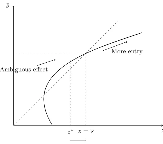
My results about simultaneous entry show that allowing for entry does not necessarily correct the strategic rationing of liquidity (measured as the spread) caused by imperfect competition among arbitrageurs. The risk-averse arbitrageurs must decide ex-ante whether to enter (and sink a fixed cost) under uncertainty about the arbitrage profitability. An increase in average shocks makes the arbitrage more profitable, and increases entry. But an increase in the volatility of shocks does not necessarily increase entry, in particular if local investors are sufficiently risk-averse. Indeed, on one hand, a higher volatility makes the arbitrage more risky, which hurts the risk-averse arbitrageurs, and on the other hand, it increases local investors’ willingness to hedge their exposure to liquidity shocks (indirect effect), and thus the arbitrage profitability. The first effect dominates and reduces entry if the risk-bearing capacity is small (highly risk-averse investors), and / or the market is concentrated, and / or if volatility is small relative to the average shock (most likely, a large shock will hit the market). Hence entry depends on the “market structure of risk-bearing capacity” (Pritsker, 2009). These results imply that, all else equal, the number of arbitrageurs may first decrease or be stable and then increase along the northeastern direction of the mean-variance frontier of arbitrage opportunities (Figure 1.1).
Once arbitrageurs are in place, their ability to move prices can help them limit future entry, in particular if entry costs are high for new arbitrageurs, and even if the arbitrage is risk-free. Deterring new entrants requires to decrease the profitability of the arbitrage, i.e. by reducing the spread between A- and B-asset prices more quickly. This contradicts arbitrageurs’ objective to decrease the spread only gradually. When entry costs are suffi-ciently large for the entrant, the cost of deterrence is low for incumbents. As entry costs 6Similarly, there is anecdotal evidence that Leland and Rubinstein’s portfolio insurance strategy became
decrease, arbitrageurs must tackle the mispricing more aggressively ex-ante, which increases liquidity and the speed of arbitrage. In this sense, the arbitrage is contestable and the mere threat of entry improves market efficiency. As entry costs decrease further, this deterrence strategy becomes very costly as incumbent arbitrageurs must bear the cost of their adverse price impact. As a result, they engage in less aggressive preemptive buying and let the new arbitrageur enter.
When entry occurs in equilibrium, market liquidity improves along two dimensions. First, arbitrageurs keep trading more aggressively than without entry threat, which decreases the spread. This effect is consistent with evidence presented by Tufano (1989), who shows that intermediaries launching new financial products charge nearly competitive prices even during the early stages where they enjoy a monopolistic position in the product. Second, local investors’ current demand becomes more elastic as they rationally anticipate a more favourable market structure in the future. This leads to an increase in market depth and shows that with low entry costs, an improvement in market depth should be a leading indicator of an increase in the number of arbitrageurs. More generally, this result highlights a key feature of the model: market depth is endogenously determined by the current and anticipated market structure, as arbitrageurs’ market power and its evolution determine the risk-sharing opportunities available to local investors, and thus the prices at which they are willing to absorb arbitrageurs’ trades.
This paper introduces time-varying and uncertain shocks and an endogenous market structure in models where large investors competing `a la Cournot trade with a competitive fringe of investors (e.g. DeMarzo and Urosevic, 2007, Pritsker 2009).7 The time-variation in shocks generates time-variation in the arbitrage profitability and encompasses “gradual arbitrage”, as in Oehmke (2010), with the difference that the market depth is endogenous. Time variation in shocks also generates a novel sign inversion effect, in which arbitrageurs prevent prices from converging. Arbitrageurs’ destabilizing behaviour arises as an endoge-nous response to the deterioration of the arbitrage profitability. This is in contrast to the predatory trading literature, where arbitrageurs can be destabilizing as a response to the need of other traders to reduce their positions, or to induce them to do so (Brunnermeier and Pedersen, 2005, Attari, Mello and Ruckes, 2006, Fardeau, 2011a).
The analysis of arbitrageurs’ entry in the literature has been either informal (e.g. Shleifer 7There is another class of dynamic models of imperfectly competitive trading without competitive fringe:
and Vishny 1997, Kondor 2009) or based on risk-neutral arbitrageurs (Oehmke, 2010, Zi-grand, 2004 and 2006). Allowing for risk-averse arbitrageurs generates new effects such as the non-monotonic relationship between entry and volatility conjectured by Shleifer and Vishny. More generally, the model shows that entry decisions depend on the interaction between the market structure and the risk-bearing capacity of all market participants. Pritsker (2009) highlights the role of the “market structure of risk-bearing capacity” in a related paper about large investors, but does not consider entry.
Sequential entry of arbitrageurs has - to the best of my knowledge - not been studied in an asset pricing context. While the literature has traditionally focused on information asymmetry and traders’ risk-aversion (or inventory effects) as determinants of market depth, the model highlights market structure and its potential evolution as a new determinant of market depth. Sequential entry and contestability are the subjects of classic papers in Industrial Organization (e.g. Fudenberg-Tirole, 1987, Baumol, 1982).8 In a financial market,
it is interesting to see that the anticipations of consumers (here local investors) of the product (liquidity) play an important role and make the equilibria self-fulfilling. For instance, the mere anticipation of entry improves market depth, which makes it harder for arbitrageurs to deter new traders from coming in. In other words, while classic IO papers typically assume that there exist a representative consumer with a continuum of asset valuation, here the elasticity of the liquidity demand (price impact) is endogenous. It affects and is affected by the firms’ (i.e. arbitrageurs) strategic entry decisions.
Some predictions of the model are observationally equivalent to predictions delivered by limits of arbitrage models.9 In particular, both types of models predict that assets with identical cash-flows and risks can trade at different prices and that the spread between these assets should decrease over time. The drivers of these effects are imperfect competition on one hand, and capital constraints on the other hand, therefore it should be empirically possible to disentangle these theories. Ruf (2011) shows that both effects matter to explain the skewness risk premium in options market.
Imperfect competition among financial intermediaries (market-makers) is the subject of an extensive literature in market microstructure (e.g. Dennert, 1993, Biais, Martimort and 8Note that simultaneous entry is also studied in the literature on non-competitive foundations of general
equilibrium. See Zigrand (2004) and references therein.
9Some examples of this extensive literature include Shleifer and Vishny (1997), Xiong (2001) , Kyle and
Rochet, 2000). The key difference with these papers is that I assume that all information is public, which allows me to isolate the effect of market power on liquidity. Instead, Den-nert considers price competition in a framework were market-makers face adverse selection. Further, in his model, market-makers post quotes first, while here arbitrageurs compete in quantities taking local investors’ schedules as given. In Biais et al., market-makers supply liquidity by posting limit order schedules, whereas in my set-up arbitrageurs submit market orders (Cournot competition).
I proceed as follows. In section 1.2, I describe the model. I solve for the equilibrium with a given market structure in Section 1.3. In Section 1.4, I endogenize the number of arbitrageurs. Section 1.5 concludes. All proofs and figures are in the appendix.
1.2
A model of imperfectly competitive arbitrage
The model features two markets for identical assets (AandB). Some investors (arbitrageurs) can trade freely across both markets, while others (local investors) are constrained to trade in only one market, a building block similar to Gromb and Vayanos (2002). A key difference with this paper is that arbitrageurs are imperfectly competitive and are not financially constrained.
1.2.1
Set-up
Assets and timeline. The economy has three periods 0, 1 and 2, and consists of two identical risky assets (A and B) in zero net supply. The risky assets pay off a liquidating dividend at time 2, D2 = D+1+2, where t are iid normal variables with mean 0 and
varianceσ2. The fundamental shocks1 and2 are realized at time 1 and time 2, respectively,
and are publicly observed. I denote Dt = Et(D2), the conditional expected value of the
dividend. There is also a risk-free asset in perfectly elastic supply with returnr normalized to 0. Trading takes places at time 0 and time 1 and consumption at time 2.
fornto change endogenously over time through the entry of new arbitrageurs at time 1. Arbi-trageurs have CARA utility with absolute risk-aversion coefficientb: U(C2i) =−exp (−bC2i),
with i = 1, ..., n. Arbitrageurs have no endowment in the risky assets. Importantly, local
investors are restricted to trade their local risky asset, while arbitrageurs can trade all risky assets. In other words, markets A and B for the risky asset are completely segmented. All investors have access to the risk-free asset.
Liquidity / supply shocks. The local investors in market k receive endowment shocks
sk01 at time 1 and sk12 at time 2. I assume that shocks are opposite across markets: sAt = −sBt = st, for t = 0,1. The shocks are correlated to the payoff of the risky asset, and
are opposite across markets. Since risky assets are identical and A- and B markets, local investors could achieve perfect risk sharing by trading with each other in the risky asset. However market segmentation prevents direct trading between local investors and creates a trading opportunity for arbitrageurs, who can intermediate trades by buying from investors with low valuation (in market A) and selling to investors with high valuation (in market B). Doing so, arbitrageurs will contribute to integrate markets A and B and provide liquidity to local investors. Thus the endowment shocks create a demand for liquidity and constitute the “supply” of assets available for arbitrage from the point of view of arbitrageurs.
I consider two situations. In the first situation, all traders know in advance the values of
s0 and s1, i.e. they know the magnitude of the supply. In this case, the trading opportunity
corresponds to a textbook arbitrage since it involves no risk. Allowing for s0 to be different
froms1 helps me understand how changes in supply affect the dynamics of arbitrage. Many
results can be derived in this simple risk-free arbitrage case, in particular gradual arbitrage and sign inversion. The second situation is closer to a real-life arbitrage opportunity, because it entails some risk. I assume that the magnitude of the second shock, s1, is random from
the point of view of time 0 for all traders: s1 is normally distributed with mean ¯s1 and
variancez2
1, and is independent of t. Thisrisky arbitrage case allows me to investigate how
uncertainty affects the dynamics of strategic arbitrage and arbitrageurs’ risk-management strategies.
arbitrageurs smooth out the temporary order imbalances by holding the asset in between subperiods. In the second interpretation, arbitrageurs can be thought of as large hedge funds or prop trading desks chasing mispricings between identical or quasi-identical assets, such as on-the-run and off-the-run Treasuries, Siamese stocks (e.g. Royal Dutch and Shell), etc. Long-Term Capital Management (LTCM) is a standard example of this kind of traders.10
The shocks affecting local investors can stem from institutional or regulatory frictions. For instance, index trackers and mutual fund managers must rebalance their portfolios following index additions or deletions because of benchmarking constraints. Negative shocks in one as-set can force portfolio managers of open-ended funds to sell other asas-sets to meet redemptions, etc.11
1.2.2
Maximization problems
Local investors. At time 2, local investors consume their entire wealth:
C2k=W2k =Y1kD2+E1k, k=A,B
In this equation, Yk
1 and E1k represent investors k’s end-of-period positions in the risky and
risk-free assets at time 1. That is, local investors in market k enter period 2 at which they only consume with a position Yk
1 in the risky asset and E1k in the risk-free asset.12 I denote
yk
t the time t trade in risky asset k and pkt its price. The law of motion of positions is:
Yk
t =Ytk−1 +ytk for the risky asset and Etk = Etk−1 −ykt +sktt+1, for the risk-free asset, for
k =A, B.13 The local investors’ dynamic budget constraint follows:
Wtk+1 =Wtk+Ytk pkt+1−pkt+sktt+1, k=A,B (1.1)
This equation shows that local investors’ wealth changes either because of capital gains,
Yk
t pkt+1−pkt
, or because of shocks, sk
tt+1. The local investors maximize the expected
10LTCM also provide a good illustration of the issue of size and market impact. As P´erold (1999) puts it:
“The firm had also experienced many instances in which prices moved adversely while LTCM was attempting to exit a position after it had converged, suggesting that the firm’s trades were having a larger market impact” (than previously).
11Gromb and Vayanos (2010) provide more details and other examples. 12Observe also that at time 2, each market is perfectly liquid, so thatpk
2 =D2. 13Since local investors have CARA preferences, we can set their initial endowmentEk
−1= 0 without loss
utility of consumption subject to the dynamic budget constraint:
for k=A, B, max
(Yk t )t=0,1
E u C2k
(1.2)
s.t. Wtk+1 = Wtk+Yt pkt+1−p
k t
+sktt+1
Arbitrageurs. Arbitrageurs face a different budget constraint because they can trade in both markets. Their final wealth W2i is equal to:
W2i =B1i + X
k=A,B
X1i,kD2, i= 1, . . . , n (1.3)
Note thatXti,k and xi,kt represent the arbitrageuri’s position and trades at timetin asset k, and are related as follows: Xti,k =Xti,k−1+xi,kt . The position in the risk-free asset evolves as:
Bi
t =Bti−1−
P
k=A,Bx i,k
t pkt. Therefore the dynamic budget constraint is:
Wti+1 =Wti+ X
k=A,B
Xti,k pkt+1−pkt
, i= 1, . . . , n
As in Gromb and Vayanos (2002), I will focus on equilibria in which arbitrageurs take opposite positions in each market: for t= 0,1, xi,At =−xi,Bt =xit. Given that assets A and
B are both in zero net supply, this implies that arbitrageurs do not bear any aggregate risk.14 With opposite positions in markets A and B, the dynamic budget constraint becomes:
Wti+1 =Wti+Xt pBt −pAt − pBt+1−pAt+1
=Wti+Xt(∆t−∆t+1), i= 1, . . . , n (1.4)
The arbitrageur’s dynamic budget constraint shows that their wealth changes via capital gains in the arbitrage. The arbitrageurs’ problem is to choose tradesxit,t= 0,1, to maximize their expected utility of consumption subject to (1.4) and the price schedules for assets A and B. The price schedules are derived from local investors’ inverted demand schedules, and imposing market-clearing:
Ytk+
n X
i=1
Xti,k = 0, k =A, B, t= 0,1 (1.5)
14In the more general case where the supply is different from zero, an additional risk-sharing motive would
The price schedules map the effect of arbitrageurs’ trades into the price in each market. That is, a price schedule represent the market-clearing price at which the competitive fringe of local investors in each market is ready to trade all possible quantities submitted by arbitrageurs. Hence arbitrageurs will internalize their price impact in each market when choosing their positions in the risky asset. Of course, the specific form of the local investors’ demand schedules also depends on the liquidity / supply shocks, and in particular, on whether future shocks are known in advance or are random. In the next section, I derive the equilibrium in the risk-free and risky arbitrage cases.
1.3
Equilibrium with risk-free and risky arbitrage
In this section, I solve for local investors’ and arbitrageurs’ equilibrium strategies, taking the number of arbitrageurs as given. When the arbitrage is risk-free, the price dynamics depend crucially on whether the supply shocks are constant or not. The risky arbitrage case allows me to analyze in details arbitrageurs’ risk-management strategies.
1.3.1
Risk-free arbitrage
Price schedules. Here I assume that s0 and s1 are positive shocks and are known in
advance by all market participants. As a first step, it is useful to look at the price schedules faced by arbitrageurs at time 1. In our standard CARA-normal framework, local investors’ demand in market A is:
Y1A= E(D2)−p
A
1
aσ2 −s1 (1.6)
Local investors in market A experience a positive shock s1, which reduces their demand
for asset A. In market B, local investors have similar demand functions (in pB1), except that they experience an opposite shock, increasing their demand for asset B. Using the assumption of opposite positions in markets A and B, and imposing market-clearing (1.5), these demand functions generate the following price schedules pk
shorthand Q1 =
Pn
i=1X1i:
pA1 (Q1) = E1(D2)−aσ2
"
s1−
n X
i=1
X1i
#
=E1(D2)−aσ2
"
s1−
n X
i=1
xi0−
n X
i=1
xi1
#
pB1 (Q1) = E1(D2) +aσ2
"
s1 −
n X
i=1
X1i
#
=E1(D2) +aσ2
"
s1−
n X
i=1
xi0−
n X
i=1
xi1
#
Note that we used the assumption that arbitrageurs have no preexisting position in any of the risky assets, i.e. xi
0 = X0i. Combining the two schedules, we get the following schedule
for the arbitrage spread, ∆1(Q1) = pB1 (Q1)−pA1 (Q1):
∆1(.) = 2aσ2
"
s1−
n X
i=1
xi0−
n X
i=1
xi1
#
(1.7)
The schedule has an intuitive form. The first component, 2aσ2s
1 is the price wedge that
would prevail between assets A and B in the absence of trading. That is, A-investors, who experience a positive liquidity (supply) shock, would have to hold all the additional supply and would thus value the asset at a discount aσ2s
1 relative to its expected payoff E1(D2).
B-investors would value the risky asset at exactly the opposite premium, as they experience a negative shock of similar magnitude. Hence in total the price wedge would be 2aσ2s1,
increasing with the risk of the asset,σ2, the risk-aversion of local investors a, and the size of the liquidity shocks1. The second component of (1.7) represents the impact of arbitrageurs’
trades. Arbitrageurs can bring prices of assets A and B closer by setting up a long position in the spread (corresponding to a long position in asset A minus a short position in asset B). Arbitrageurs’ price impact, |∂∆1
∂xi 1
| = 2aσ2, depends on local investors’ risk-aversion and the
risk of the fundamental.15 When they are more risk-averse, local investors are more reluctant
to hold the risky asset, and thus will require larger price concessions when trading, resulting in a larger price impact.
Equilibrium strategies and spreads. To illustrate the strategic choice faced by arbi-trageurs, note that because arbitrageurs set up opposite positions, their objective at time 1 boils down to maximizing the trading profit, xi
1∆1(.), where ∆1(.) is given by (1.7) and
depends not only on arbitrageuri’s trade, xi
1, but also all other arbitrageurs’ trades
P
−ix
−i
1 ,
with P
−ix
−i
1 +xi1 =
Pn
i=1x
i
1, and on the positions established at time 0,
P ix
i
0. Hence at
other arbitrageurs’ on the spread. In the appendix, I work backwards to derive arbitrageurs’ optimal trading strategies and obtain the following result:
Proposition 1 In the risk-free case, there is a unique (symmetric) equilibrium in which
arbitrageurs’ trades in market A are:
xi0 = x0 =
1
φn
s0+
n−1
(n+ 1)2φn
s1 (1.8)
xi1 = x1 =−
n
(n+ 1)φn
s0+ ¯φns1, (1.9)
The equilibrium spread is:
∆0 = 2aσ2
ψns0+ ¯ψns1
(1.10) ∆1 = 2aσ2
− n
(n+ 1)φn
s0+ ¯φns1
(1.11)
with φn =
n3+ 4n2+ 3n+ 2
(n+ 1)2 ; ¯φn = 1
n+ 1 −
n(n−1)
(n+ 1)3φn
ψn =
n2+n+ 2
n3+ 4n2+ 3n+ 2; ¯ψn =
3n2+ 5n+ 2
n3+ 4n2+ 3n+ 2
Gradual arbitrage with constant liquidity shocks (s0 =s1 =s)
To gain intuition into the equilibrium, it is useful to consider the special case s0 = s1 =s,
withs >0, to fix ideas. Then arbitrageurs’ trades arexi
0 =κ0,ns andxi1 =κ1,ns, with for all
n ≥ 1, κ0,n ≡ φn1
1 + n−1
(n+1)2
∈ ]0,1[ and κ1,n ≡ −(n+1)nφn + ¯φn ∈ ]0,1[. Further, the total
purchases are:
n X
i=1
xi0 =nκ0,ns < s and
n X
i=1
xi1 =nκ1,ns < s
Hence arbitrageurs never fully absorb the asset supply caused by the liquidity shock in each market. As a result, the spreads between A- and B-asset prices remain strictly positive in equilibrium:
Why does competition not eliminate the mispricing as soon as n > 1? It can be seen from the time-1 objective:
max
xi 1
xi1∆1(.) = max
xi 1
2aσ2xi1 s− n X
i=1
xi0−X
−i
x−1i−xi1
!
(1.12)
For a given liquidity shock s, given other arbitrageurs’ tradesP
−ix
−i
1 , and initial positions
P ix
i
0, arbitrageurihas no interest to buy the entire residual supply, s−
Pn
i=1x
i
0−
P
−ix
−i
1 ,
for he would then close the spread and make a zero profit on his trade. Instead, his best response, from the first-order condition of problem (1.12), is to trade half the residual supply:
xi1 = s−
Pn i=1xi0−
P
−ix
−i 1
2 . Since each arbitrageur has the same impact on the price, all
arbi-trageurs play a symmetric role, and in the unique (subgame) equilibrium, all arbiarbi-trageurs trade the same quantity, xi1 = s−
Pn i=1xi0
n+1 .
This quantity is negatively related to the arbitrageurs’ first period trades, Pn
i=1xi0.
In-deed, to keep the spread open, arbitrageurs need to limit their price impact, which is perma-nent, as shown by equation (1.7). The reason why price impact is permanent is that for local investors in, say market A, who have a low valuation for the asset, selling the asset to arbi-trageurs helps insure against the first liquidity shock, but also, to some extent, against the second liquidity shock. Indeed the second shock is also correlated with the asset payoff (and has same constant part s). Hence hedging at time 0 can serve as proxy hedging for time 1. Thus there is some substitutability between insurance (liquidity) received from arbitrageurs at time 0 and that received at time 1. The fact that the liquidity received by local investors at time 0 “durably” reduces their hedging demand at time 1 erodes arbitrageurs’ market power. Hence providing liquidity by intermediating trades across markets bears resemblance to the provision of a durable good by a monopolist and is subject to similar Coasian dynamics.16
The equilibrium implication of these dynamics is that when the profitability of the arbi-trage is constant over time (s0 =s1 =s), arbitrageurs increase their positions only gradually.
This results in gradual convergence of prices towards the fundamental, even more so if the market is particularly concentrated. When competition increases, each arbitrageurs buys 16Coase (1972)’s intuitions about the durable goods problem for a monopoly have been formalized by
(sells) a smaller amount in market A (B). However the aggregate quantity traded in equi-librium increases, as Figure 1.3 shows. In the limit, arbitrageurs fully intermediate trades between A- and B-investors and the equilibrium spread converges to zero. The following corollary summarizes these results:
Corollary 1 Suppose s0 =s1 =s, then
• the spread is always positive and decreases with the number of arbitrageurs at time 0 and time 1: ∂∆t
∂n <0, t= 0,1,
• the spread decreases over time: ∆2 = 0 <∆1 <∆0,
• and it decreases faster as n increases: ∂ h
∆1−∆0
∆0 i
∂n <0.
• When n→ ∞, the arbitrageurs absorb the entire liquidity shock at time 0 and time 1, and the spread converges to zero: limn→∞∆t = 0, t= 0,1.17
These results generalize the idea of “gradual arbitrage” developed in Oehmke (2010) in a setting where the price schedules against which arbitrageurs trade are endogenous. Owing to imperfect competition, arbitrageurs can slow down the speed of arbitrage across markets, resulting in gradual convergence of prices towards the fundamental value.18 Said differently,
as arbitrageurs will set better prices in the future, it is optimal for local investors to hold some of the excess supply created by their liquidity shock. As Oehmke points out, this mech-anism can account for the observed slow reversal of prices towards fundamentals following shocks documented, for instance, by Mitchell, Pulvino and Stafford (2002) in the convertible arbitrage market, and Coval and Stafford (2007) in the equity market.
Time-varying price impact. In Oehmke’s model, as in other related papers in the liter-ature (e.g. Carlin, Sousa-Lobo and Viswanathan, 2007, Brunnermeier and Pedersen, 2005), arbitrageurs trade against an exogenous price schedule with constant price impact coeffi-cient.19 With endogenous price schedules, the arbitrageurs’ price impact is no longer constant
over time. It decreases as time passes and depends on the market structure:20
17Note that this result does not depend on the assumptions
0=s1=s. 18In Oehmke’s model, the arbitrage is risky but arbitrageurs are risk-neutral.
19As some of these models are framed in continuous time, there is also a temporary price impact component
that helps pin down the equilibrium speed of trading.
20This result is general and does not depend on the assumption that shocks are constant over time, or
Corollary 2 Price impact decreases over time, even more so if the market is concentrated
(n small):
• At time 1, arbitrageurs’ price impact is |∂∆1 ∂xi
1
|= 2aσ2 (i= 1, . . . , n)
• At time 0, the equilibrium spread schedule is
∆0(Q0) = 2aσ2
"
s0+
s1
(n+ 1) −
n+ 2
n+ 1
X
i xi0
#
, (1.13)
i.e. arbitrageurs’ price impact is |∂∆0 ∂xi
0
|= 2aσ2n+2
n+1 >|
∂∆1 ∂xi
1 |.
The spread schedule at time 0 has two components. The first component, 2aσ2s
0+(ns+1)1
, is the spread that would obtain if arbitrageurs did not trade at time 0 in equilibrium. It is increasing in s0 and s1, because local investors anticipate that risk-sharing at time 1 will be
limited due to arbitrageurs’ market power. Indeed, an increase in market competitiveness improves risk-sharing and in the limit eliminates s1. The second component represents the
arbitrageurs’ price impact, aσ2n+2
n+1. Two opposite effects determine the evolution of price
impact over time. First, given that new information accrues over time, the conditional variance of the asset payoff is decreasing over time as uncertainty realizes. This implies that local investors in each market are “more risk-averse” at time 0 than at time 1. Since the variance of each innovation t is constant over time, price impact should be twice as large
at time 0 than at time 1. This is not the case, however, because a second effect tends to reduce price impact.21 As local investors anticipate that arbitrageurs will provide further liquidity at time 1, they understand that they will have another trading opportunity to share risk, and this reduces their effective level of risk-aversion ex-ante. Said differently, local investors are less desperate to receive liquidity if they anticipate that more liquidity is coming later on.22 The more concentrated the market is, however, the more rationed
liquidity will be (aσ2n+2
n+1 is maximal for n = 1), and therefore price impact is higher at
time 0 if the market is concentrated - or, more precisely, expected to remain concentrated.23
Note that at time 1, arbitrageurs’ price impact depends only on risk-aversion and not on the market structure. This is because at time 2, the asset pays off, which is equivalent to
21It is easy to see that, indeed for anyn≥1, 2aσ2n+2
n+1 <4aσ 2.
22As noted above, these Coasian dynamics crucially depend on the fixed horizon of the model, and
arbi-trageurs’ inability to commit to trade only once.
23In Section 1.4.2, I allow for a new arbitrageur to enter at time 1 upon sinking a fixed cost, therefore
restoring perfect liquidity in the market. If the market was perfectly competitive also at time 1, the market structure adjustment of time 0 price impact would disappear, and price impact would be constantaσ2nn+2+1 →aσ2.
This dynamic “contamination” of illiquidity from period 1 to period 0 is therefore due to imperfect competition and the limited risk-sharing that it implies. The same dynamic effect is present in Rostek and Weretka (2010), who study a setting with n strategic arbitrageurs and no competitive fringe. Their model, however, predicts that price impact should increase over time, because only the second effect, stemming from the opportunity to retrade and diversify risk further in the future, is present. The comparison of our results therefore reveals that the direction of change of market depth over time - whether it increases or decreases over time - should depend not only on the market microstructure but also on the uncertainty surrounding the asset payoff. Here the model predicts that price impact should decrease as the date of the asset payoff approaches, but even more so if only a few large arbitrageurs are active in the trade.
Optimal execution with endogenous market depth. An interesting implication of the time-varying price impact is that a monopolistic arbitrageur does not equally split his trade across periods: for n = 1, κ0,1 = 25 > κ1,1 = 103 , i.e. x0 > x1. (More generally, for
an arbitrary number of arbitrageurs, x0 > x1) This is a key difference with the literature
on optimal execution of large orders (e.g. Bertsimas and Lo, 1998), which shows that with constant price impact, it is optimal for a monopolistic trader to break up orders equally over time. Thus the model highlights that in concentrated markets, optimal order execution and market depth are jointly determined and depend on the deep characteristics of the market, such as investors’ risk-aversion, asset volatility and the market structure.
Sign inversion with changing supply shocks (s0 ≥0, s1 ≥0)
The case where the supply of arbitrage changes over time brings further insight into the mechanisms and generates new predictions. First, proposition 1 shows that the time-0 trade (1.8) depends on both s0 and s1, unless there is a single arbitrageur. This shows that when
competition increases, the pressure to share risk with local investors increases, so that local investors are able to start hedging their future risk. Note that, independently of the number of arbitrageurs, the time-0 equilibrium spread always depends on both s0 and s1, because
Sign inversion. Changes in shocks, i.e. variation in the arbitrage supply, generates sign inversion: when both shocks are positive, ∆1 may become negative, even though s1 ≥ 0.
Remember that a positive shock implies that A-investors should value the asset less than B-investors, suggesting that ∆1 should be positive. Note from equation (1.10), that ∆0 is
always positive with s0 ≥ 0 and s1 ≥ 0. The sign of the spread can switch over time if the
profitability of the arbitrage deteriorates:
Corollary 3 Suppose that s0 and s1 are positive.
• At time 0, the spread is always positive and decreases with the number of arbitrageurs:
∂∆0 ∂n <0. • At time 1:
– The spread is negative if and only ifs1 is small enough relative to s0: ∆1 ≤0 ⇔
s1 ≤αns0, with 0< αn <1.
The condition for sign inversion is that liquidity shocks decrease sufficiently over time, i.e. that the arbitrage profitability decreases sufficiently. An interpretation of the condition is that sign inversion may occur in the aftermath of a large shock, and close to the time where assets mature, or where convergence occurs for exogenous reasons (e.g. when an on-the-run bond is close to becoming off-the-run). Hence the model predicts that sign inversion should occur following periods of low liquidity (or equivalently large price divergence).
To understand the intuition of the mechanism, consider an example in which s0 > 0
and s1 = 0. In this case, local investors in market A initially short the asset, receiving
partial insurance against the positive supply (liquidity) shock from arbitrageurs who limit the amount they buy thanks to market power. At time 1, since there is no reason to hedge anymore (s1 = 0), local investors seek to close their hedge by buying back the asset (indeed,
yA
1 >0). However, arbitrageurs continue to limit liquidity at this time, so that local investors
cannot fully close their short position. This pushes the price of asset A above its expected value. As a consequence, local investors remain short, YA
1 < 0, as one can see by setting
s1 = 0 in equation (1.6). This is optimal since the price of asset A will (on average) drop
even if the spread sign inverts, because their profit depends on the fact that prices do not converge and not on the sign. As I show in the proof of Proposition 1, the trading profit at time 1, x1∆1, is equal to 2aσ2
(s1−Pni=1xi0) 2
(n+1)2 , with x1 =
s1−Pni=1xi0
n+1 and ∆1 = 2aσ
2s1−Pni=1xi0
n+1 .
Hence, arbitrageurs care about the magnitude of the mispricing rather than the sign.
As Lemma 3 shows, s1 does not have to be zero, but small enough relative to s0.
Intu-itively, the need to revert the hedge must simply be large enough for the spread to invert at time 1. Hence, the time-1 spread can turn negative even though all liquidity shocks imply that it should be positive. Interestingly, it is precisely when local investors’ demand pres-sures decrease that arbitrageurs push the spread to invert. Hence it is when asset prices should converge towards their fundamental value that arbitrageurs cause a breakdown of the intuitive relationship between A-and-B asset prices. What causes this breakdown is that arbitrageurs limit liquidity both when local investors need to sell and to buy. Because it is driven by the variation in the arbitrage profitability, this result is not present in Oehmke (2010) in which only the initial shock matters.24
This result may shed light on recent puzzling evidence about closely-related assets. Indeed several standard and intuitive relationships broke down in the aftermath of the 2007-2009 financial crisis. For instance, the 7-and 10-year swap spread turned negative for the first time in 2010 (Business Week, 23/03/2010). Uninsured municipal bonds became more expensive than similar insured bonds issued by the same city also in 2010 (Bergstresser et al., 2011).25
The extent of the mispricing, in particular in the municipal bond market, makes standard explanation implausible. For instance, a negative swap spread may be justified by heightened concerns about sovereign risk. Similarly, concerns about monoline insurers may reduce the premium attached to insured bonds to zero. However, it is hard to see how it could generate a negative premium. Although these explanations may be partially correct, the model offers a single complementary mechanism based on market structure and easing of demand pressures.
24Specifically, Oehmke considers the time-inconsistent trading strategies of strategic arbitrageurs facing
two exogenous demand curves for the same asset. Since the strategy is solved ex-ante, all results are a function of the initial liquidity shock, which eliminates the possibility of time variation in the arbitrage profitability.
25Inflation-protected Treasuries also became cheaper than similar nominal bonds (Pflueger and Viceira,
1.3.2
Risky arbitrage
In this section, I assume that s1 is not known at time 0. Investors only know that it is
normally distributed with mean ¯s1 and variance z12. I also make the following assumption
about the parameters: Assumption 1 a2σ2z2
1 < (n+1)2
2n+1
Since the second shock is random from the point of view of time 0, the arbitrage is no longer risk-free. Therefore, even if arbitrageurs can eliminate all fundamental risk by taking opposite positions in assets A and B, they face uncertainty about the future profitability of the arbitrage. As in standard noise trader risk models, the potential deepening of the mispricing is short-lived, and the prices assets A and B converge at time 2 when the assets pay off. This risky arbitrage case allows me to delve more deeply into the mechanisms and to analyze arbitrageurs’ risk-management strategies.
Price schedules and equilibrium
At time 1, the problem is not different from the risk-free case. However at time 0, all investors face uncertainty about the magnitude of the future liquidity shock. I show in the appendix that at time 0, the spread schedule faced by arbitrageurs is the following:
∆0(.) = 2aσ2
"
s0+
¯
s1
(n+ 1)ra
− n+ 2
n+ 1(1 +φa)
X
i xi0
#
, (1.14)
with φa =
a2σ2z2 1
(n+ 1)2ra
and ra= 1−a2σ2z12
2n+ 1
(n+ 1)2 (1.15)
There are two key differences with respect to the risk-free case, in which the schedule is given by equation (1.13), which I reproduce here for convenience: ∆0(.) = 2aσ2
h
s0 +(ns+1)1 −nn+2+1
P ixi0
i
. The first part of the schedule, s0+ (n+1)s¯1 ra, represents the price divergence that would
pre-vail in equilibrium in the absence of trade. Given that ra < 1, we have: s0 + (n+1)¯s1 ra >
E0
h
s0+(ns+1)1
i
, which captures the effect of convexity, as in Jensen’s inequality. The second part represents arbitrageurs’ price impact. It increases by a factor 1 +φa>1 relative to the
Uncertainty about future liquidity shocks also affects arbitrageurs’ strategies at time 0, both through their own risk aversion and through the change in the price schedules. The different channels appear clearly in their value function:
Proposition 2 At time 0, the arbitrageurs’ value function is given by
J0i = max
xi 0
−r−
1 2
b exp
"
−2baσ2 xi0∆ˆ0+ (1−φb)
(P ix
i
0) 2
(n+ 1)2 − ¯
s1
(n+ 1)2rb
2X
i
xi0−s¯1
!!#
where ∆ˆ0 =
∆0(.)
2aσ2 , rb = 1 +
4abσ2z2 1
(n+ 1)2 and φb =
4abσ2z2 1
(n+ 1)2rb
(1.16)
Arbitrageurs’ value function is made of three components:
1. Their time-0 trading profit 0, xi
0∆ˆ0, i.e. quantity times (normalized) price gap ˆ∆.
2. The time-1 continuation profit, in which we can distinguish two parts, depending on their relation to risk aversion:
(a) The first part, (1−φb)
(P ixi0)
2
(n+1)2 , is decreasing in arbitrageurs’ risk aversionb, and
more generally in z2
1, σ2, and a. Hence I will refer to it as the precautionary (or
hedging) motive. The coefficient φb measures by how much arbitrageurs reduce
their aggressiveness in tackling the arbitrage gap at time 0 for fear of facing too much risk at time 1. Note that φb depends on the product of a and b because
an increase in local investors’ risk-aversion makes them more reluctant to hold the risky asset and thus restricts arbitrageurs’ risk-sharing opportunities. The hedging motive is, perhaps surprisingly, increasing in the total size of previous trades, P
ix i
0. This is because trading aggressiveness at time 0 works as an
indirect hedge against large shocks at time 1 by reducing the spread permanently. The strength of the hedging motive also depends on the number of arbitrageurs. A change in market structure has two conflicting effects:
Corollary 4 At time 1, when the number of arbitrageurs increases, there is
• a business-stealing effect: ∂ 1
(n+1)2
∂n <0, which reduces the coefficient
1−φb
(n+1)2,
The business-stealing effect always dominates the co-insurance effect, i.e. ∂
1−φb
(n+1)2
∂n <
0.
The business-stealing effect is the standard consequence of stronger competition in a Cournot setting. The co-insurance effect is positive because as n increases, risk-sharing becomes more effective: more competition means that arbitrageurs supply more liquidity and each arbitrageur benefits from this collective effect. (b) The second part of the time-1 continuation payoff represents the “strategic
mo-tive”:
− s¯1
(n+ 1)2rb
2X
i
xi0−¯s1
!
It isincreasing in arbitrageurs’ risk-aversion b and decreasing in previous trades, as arbitrageurs have an incentive to strategically limit their positions at time 0 to be able to fully exploit the arbitrage opportunity later. The key driver of the strategic motive is the expected level of arbitrage risk ¯s1 instead of the risk of the
arbitrage riskz2
1, as explained in more details below.
Proposition 3 When arbitrage is risky, there is a unique (symmetric) equilibrium charac-terized by:
xi0 =
s0+ (n+1)¯s1 ra − (n+1)2¯s12 rb
φn+ (n+ 2)φa+ 2nφb
(1.17)
xi1 = s1−
P ix
i
0
n+ 1 (1.18)
The equilibrium spread between asset B and asset A is
∆0 = 2aσ2
Φa
s0+
¯
s1
(n+ 1)ra
+ (1−Φa)
2¯s1
(n+ 1)2rb
, with Φa ∈[0,1] (1.19)
∆1 =
2aσ2
n+ 1
−n
ds0+
s1−
n
(n+ 1)2
(n+ 1)rb−2ra drarb
¯
s1
(1.20)
with d=φn+ (n+ 2)φa+ 2nφb.
To understand the mechanisms, it is helpful to decompose x0 in two terms:
x0 =
s0+(n+1)¯s1 ra
φn+ (n+ 2)φa+ 2nφb
−
2¯s1
(n+1)2rb
φn+ (n+ 2)φa+ 2nφb
(1.21)
The first term shows that arbitrageurs buy a fraction φn+(n+2)1φa+2nφb of the expected spread that would prevail in the absence of liquidity provision (the maximum spread), s0+(n+1)¯s1ra.
This maximum spread represents the demand for liquidity addressed to arbitrageurs at time 0. Only part of this demand is served as arbitrageurs’ market power allows them to ration liquidity. Arbitrageurs serve a smaller fraction of the demand as their risk aversion
b increases, due to precautionary concerns, and as local investors’ risk aversion a increases, because arbitrageurs have a larger price impact at time 0, which prompts them to scale back their trade (as captured by the coefficientφa). What is interesting is that arbitrageurs
provide less than a fraction of the maximum spread, since the second term in (1.21) is negative. The second term captures the effect of the arbitrageurs’ strategic motive. It becomes more negative as aversion decreases. In the limit, as arbitrageurs become risk-neutral, the strategic motive is strongest:
when b→0, xi0 → s0+
¯
s1
(n+1)ra
φn+ (n+ 2)φa
−
2¯s1
(n+1)2
φn+ (n+ 2)φa
(1.22)
In fact, the strategic motive is present even in the absence of uncertainty about liquidity shocks. To eliminate uncertainty, consider the limit case where arbitrageurs are risk-neutral
b→0, and uncertainty vanishesz1 →0. Thenx0 converges to (1.8), its equilibrium quantity
when the arbitrage is risk-free (assumings1 = ¯s1):
When z1 →0, b→0, xi0 →
s0+(ns¯+1)1
φn
−
2¯s1
(n+1)2
φn
= 1
φn
s0+
n−1
(n+ 1)2φn s1
Hence in hindsight, this decomposition highlights a fact that was hard to identify when the arbitrage was risk-free. Arbitrageurs respond to their commitment problem by buying less than a fraction of the maximum spread, s0+ (n+1)s1 ra. This reduction, −(n+1)2¯s12
rb, arises
because arbitrageurs strategically refrain from tackling the spread too aggressively at time 0, in the hope that a large shock will increase the local investors’ risk-sharing needs at time 1. Arbitrageurs “speculate” more when the market is more concentrated (n small) and the expected shock ¯s1 is large. Given the partial substitutability between liquidity provision at
large liquidity needs as much as possible later on.
The strategic motive resembles the standard risk-management mechanism that arises in models where competitive arbitrageurs face financial constraints. Several papers in the limits of arbitrage literature (e.g. Shleifer and Vishny, 1997, Gromb and Vayanos, 2002) show that financially-constrained arbitrageurs refrain from taking on too much risk early on in order to save capital and be able to exploit potentially large price discrepancies at later periods. This mechanism is based on the limited amount of capital available to competitive arbitrageurs in the short-term. Here the effect is related to market power and is a response to the perfect foresight of local investors, which erodes arbitrageurs’ market power as in the classic durable goods monopoly problem. Interestingly, the strategic motive is strongest when arbitrageurs are risk-neutral, precisely when they are most likely to aggressively tackle arbitrage opportunities.
Since the precautionary and the strategic motives have opposite dependence on arbi-trageurs’ risk aversion, an increase in b has an ambiguous effect.
Arbitrageurs’ risk aversion and liquidity
According to Friedman (1953), speculators reduce price volatility by smoothing out tempo-rary price fluctuations. Given that this view implies a contrarian behaviour, it may seem desirable to have risk-loving arbitrageurs for markets to be efficient. This is no longer the case when arbitrageurs have price impact: the spread between assets A and B may increase as arbitrageurs become risk-neutral. On one hand, a decrease in risk aversion increases arbitrageurs’ trading aggressiveness to tackle the arbitrage. On the other hand, a lower risk-aversion makes them more likely to engage in strategic “speculation”, as shown by the following result:
Corollary 5 An increase in arbitrageurs’ risk-aversion may result in them providing more or less liquidity at time 0. There are two opposite effects:
∂xi
0
∂b =κ
−n(n+ 1)2
s0+
¯
s1
(n+ 1)ra
| {z }
precautionary motive <0
+ s¯1
d+2n
rb
| {z }
reduction in strategic motive >0
The reduction in strategic motive dominates iff s1 is large enough relative to s0:
∂xi0
∂b ≥0⇔s¯1
d− n((n+ 1)rb−2ra)
rarb
≥n(n+ 1)2s0
The following lemma shows a special case in which the strategic motive is so strong that a decrease in risk aversion does lead to an decrease in liquidity provision (and conversely, an increase in risk aversion leads to higher liquidity):
Lemma 1 Suppose that s0 → 0. If n ≤ 2 and local investors’ risk-aversion a is small
enough (or equivalently, σ2 or z12 small enough), then, following a small increase in their risk-aversion, arbitrageurs provide more liquidity, which decreases the time 0 spread and
increases the expected return of the arbitrage. This effect is stronger if they are not very
risk-averse.
Unsurprisingly, the strategic motive dominates in a very concentrated market, and even more so if arbitrageurs are not too risk-averse. Note that ifs0 is very small, on average, the
spread will decrease between time 0 and time 1, implying a negative return. As b increases, arbitrageurs increase their trade at time 0, and this reduces the time 0 spread more than the time 1 spread, leading to a less negative return.
How do arbitrageurs respond to an increase in arbitrage risk?
In the presence of arbitrage risk, it is important to understand whether arbitrageurs’ reac-tions to changes in risk are stabilizing (i.e. leading to smaller spreads), or destabilizing. In the limits of arbitrage literature, it is common to study how positions and prices respond to an increase in “noise trader risk” (Shleifer and Vishny, 1997), or demand pressures / supply imbalances (Gromb and Vayanos, 2010, Brunnermeier and Pedersen, 2009). It is shown that arbitrageurs do not necessarily increase their positions ex-ante when they face larger future shocks, and this may push prices further away from their fundamental values. Here, I analyze arbitrageurs’ responses to an increase in the level of the future shock, ¯s1, and in the
volatility of the shock z1. Surprisingly, the literature on limits of arbitrage has to the best
of my knowledge focused only on the first comparative static (dubbed noise trader risk). Corollary 6 Following an increase in the expected shock ¯s1, arbitrageurs increase their
po-sitions at time 0, but the spread nevertheless increases: ∂xi0
∂¯s1 ≥0 and ∂∆0
The two parts of the result may seem contradictory, as one would expect the increase in arbitrageurs’ positions to lead to a smaller spread. It is not the case because an increase in ¯
s1 also causes an increase in local investors’ liquidity demand, and arbitrageurs’ response,
albeit positive, is not commensurate with local investors’ increased need for liquidity. This is in particular due to the fact that an increase in ¯s1 increases the profitability of the arbitrage
butt also arbitrageurs’ strategic motive. This result contrasts with predictions in models of financially-constrained arbitrage, where an increase in positions leads to more efficient prices (e.g. Shleifer and Vishny, 1997, Brunnermeier and Pedersen, 2009).
Next, it is interesting to understand how arbitrageurs respond to increased uncertainty
about the future profitability of the arbitrage. As one would expect, increased uncertainty reduces arbitrageurs’ strategic motives and increases their precautionary motives. However, uncertainty about future profitability matters even when arbitrageurs are risk-neutral, as it affects local investors’ liquidity demand, as well as arbitrageurs’ price impact.
Corollary 7 Consider the limit case where arbitrageurs are risk neutral, i.e. b →0. Then arbitrageurs respond to an increase in arbitrage risk z12 by taking larger positions if and only if volatility is small enough and the expected shock is large enough relative to the current shock. Otherwise, arbitrageurs decrease their positions.
∂xi
0
∂z2
1
≥0 ⇔
(
a2σ2z2
1 < cn with cn< (n+1)
2
2n+1
¯
s1 ≥θn,as0
No matter how arbitrageurs respond, the spread always increases following an increase inz2 1:
∂∆0 ∂z2 1
≥0.
The result shows that even if arbitrageurs are risk-neutral, they may scale down their posi-tions when uncertainty about arbitrage profitability increases. There are two effects: first, local investors are demanding more liquidity, as the convexity effect (i.e. the need to insure against shocks) increases with z1 (see equation (1.14). This increases the arbitrage supply,
showing that the increase in liquidity demand always outweighs the increase in arbitrageurs’ positions.
Market power and spread autocorrelation
Arbitrageurs’ activity also implies a number of properties for the behaviour of the spread between assets A and B. First, one can see in Proposition 3 that at time 0, the spread is a weighted average (since Φa∈[0,1]) of the maximum spread (s0+(n+1)s¯1 ra) and arbitrageurs’
strategic motive. At time 1, the spread is decreasing in the previous shock and reflects the adjustment between the expected shock ¯s1 and its realization s1. Market power also
generates autocorrelation of the spreads at one lag:
Corollary 8 The spread has the following properties:
• Comparative statics: the current shock increases the spread.
∂∆t
∂st
>0, t= 0,1
• Serial correlation: suppose s0 is random from the point of view of time -1. Then, when
the number of arbitrageurs is finite, the half spread exhibits negative serial correlation
between time 0 and time 1:
autocov−1
∆0
2 , ∆1
2
<0
When perfect competition obtains, the serial correlation vanishes:
lim
n→∞autocov−1
∆0
2 , ∆1
2
= 0
1.4
Entry
I now turn to endogenize the number of arbitrageurs. I consider ex-ante free entry, as well as gradual entry. I assume that arbitrageurs only know the distribution of future shocks when they decide ex-ante. High ex-ante uncertainty about the profitability may in this regard reduce risk-averse arbitrageurs’ incentive to enter if there is enough risk-bearing capacity. When new arbitrageurs can enter gradually, arbitrageurs already active ca