A simple, flexible and automatic 3D calibration
method for a phase calculation-based fringe
projection imaging system
Zonghua Zhang,1,* Shujun Huang,1 Shasha Meng,1 Feng Gao,2 and Xiangqian Jiang2 1School of Mechanical Engineering, Hebei University of Technology, Tianjin, 300130, China 2Centre for Precision Technologies, University of Huddersfield, Huddersfield, HD1 3DH, UK
Abstract: An important step of phase calculation-based fringe projection systems is 3D calibration, which builds up the relationship between an absolute phase map and 3D shape data. The existing 3D calibration methods are complicated and hard to implement in practical environments due to the requirement of a precise translating stage or gauge block. This paper presents a 3D calibration method which uses a white plate with discrete markers on the surface. Placing the plate at several random positions can determine the relationship of absolute phase and depth, as well as pixel position and X, Y coordinates. Experimental results and performance evaluations show that the proposed calibration method can easily build up the relationship between absolute phase map and 3D shape data in a simple, flexible and automatic way.
©2013 Optical Society of America
OCIS codes: (150.1488) Calibration; (120.2830) Height measurements; (120.5050) Phase measurement; (110.6880) Three-dimensional sensing.
References and links
1. F. Chen, G. M. Brown, and M. Song, “Overview of three-dimensional shape measurement using optical methods,” Opt. Eng. 39(1), 10–22 (2000).
2. F. Blais, “Review of 20 years of range sensor development,” J. Electron. Imaging 13(1), 231–240 (2004). 3. Z. H. Zhang, “Review of single-shot 3D shape measurement by phase calculation-based fringe projection
techniques,” Opt. Lasers Eng. 50(8), 1097–1106 (2012).
4. Z. H. Zhang, D. P. Zhang, and X. Peng, “Performance analysis of a 3-D full-field sensor based on fringe projection,” Opt. Lasers Eng. 42(3), 341–353 (2004).
5. Q. Y. Hu, P. S. Huang, Q. L. Fu, and F. P. Chiang, “Calibration of a three-dimensional shape measurement system,” Opt. Eng. 42(2), 487–493 (2003).
6. P. R. Jia, J. Kofman, and C. English, “Comparison of linear and nonlinear calibration methods for phase-measuring profilometry,” Opt. Eng. 46(4), 043601 (2007).
7. M. Vo, Z. Wang, T. Hoang, and D. Nguyen, “Flexible calibration technique for fringe-projection-based three-dimensional imaging,” Opt. Lett. 35(19), 3192–3194 (2010).
8. L. Huang, P. S. K. Chua, and A. Asundi, “Least-squares calibration method for fringe projection profilometry considering camera lens distortion,” Appl. Opt. 49(9), 1539–1548 (2010).
9. H. Du and Z. Wang, “Three-dimensional shape measurement with an arbitrarily arranged fringe projection profilometry system,” Opt. Lett. 32(16), 2438–2440 (2007).
10. Z. H. Zhang, H. Y. Ma, S. X. Zhang, T. Guo, C. E. Towers, and D. P. Towers, “Simple calibration of a phase-based 3D imaging system phase-based on uneven fringe projection,” Opt. Lett. 36(5), 627–629 (2011).
11. Z. H. Zhang, H. Y. Ma, T. Guo, S. X. Zhang, and J. P. Chen, “Simple, flexible calibration of phase calculation-based three-dimensional imaging system,” Opt. Lett. 36(7), 1257–1259 (2011).
12. Z. Y. Zhang, “A flexible new technique for camera calibration,” IEEE Trans. Pattern Anal. 22(11), 1330–1334 (2000).
13. Jean-Yves Bouguet, “Camera Calibration Toolbox for Matlab,” http://www.vision.caltech.edu/bouguetj/calib_doc/.
14. A. Fitzgibbon, M. Pilu, and R. B. Fisher, “Direct least square fitting of ellipses,” IEEE Trans. Pattern Anal. 21(5), 476–480 (1999).
15. Z. H. Zhang, S. S. Meng, and S. J. Huang,D. J. Dorantes-Gonzalez, ed., “Simple and flexible calibration method of a 3D imaging system based on fringe projection technique” in Proceedings of 16th International Conference on Mechatronics Technology, Dante J. Dorantes-Gonzalez, ed. (Tianjin Foreign Language Electronic & Audio-Video Publishing House, Tianjin, China. 2012), pp. 101–105.
17. Z. H. Zhang, C. E. Towers, and D. P. Towers, “Time efficient color fringe projection system for 3-D shape and colour using optimum 3-frequency Selection,” Opt. Express 14(14), 6444–6455 (2006).
1. Introduction
Phase calculation-based fringe projection techniques are actively studied in academia and widely applied in industries because of the advantages of non-contact operation, full-field acquisition, high accuracy, fast data processing and low cost [1–3]. Such techniques project fringe patterns onto the measured object surface. From another viewpoint, the fringe patterns are deformed with respect to the shape of the object surface. By calculating the absolute phase in the deformed fringe pattern, a 3D shape of the object is obtained with high accuracy. Therefore, in order to obtain an accurate 3D shape, an important step is to build up the relationship between the absolute phase map and 3D shape data, known as 3D calibration [4]. Existing 3D calibration methods have complicated and hard to implement procedures in practical environments because a precise translating stage or a gauge block is required. Therefore, it is a challenging problem determining how to build up the relationship between phase map and 3D shape data in a simple, flexible and automatic way, especially out of a laboratory environment.
The reported 3D calibration methods of phase calculation-based fringe projection systems can be categorized into model-based [4,5], polynomial [6,7] and least-square [8,9] methods. All the methods need an accurately translated plate or a standard gauge block. The plate needs to be accurately positioned using a high precision translating stage, so the calibration procedure is complicated and mostly implemented on an optical breadboard in the laboratory. When a gauge block is used, the placement of the gauge should satisfy certain conditions and it is difficult to carry out the calibration procedure in the field. Therefore, the existing 3D calibration methods have complicated and hard to implement procedures limited to a laboratory environment.
We previously presented a calibration method for an uneven fringe projection 3D imaging system by using a white plate with discrete markers with known separation on the surface [10]. Later, using the same white plate and a checkerboard, a general fringe projection 3D imaging system was accurately calibrated to build up the relationship between absolute phase and depth data [11]. Although the white plate and the checkerboard can be randomly placed in the measuring volume, there are still some disadvantages: firstly, all the center positions of marker were determined by manual operation, making this method both labour intensive. Secondly, the relationship between pixel position and transverse x,y coordinates is not implemented, so it is not a real 3D calibration. Thirdly, it needs two calibration plates: a checkerboard and a white plate. Therefore, the existing calibration methods cannot automatically build up the relationship between phase map and 3D shape in an actual application field.
2. Principle and method
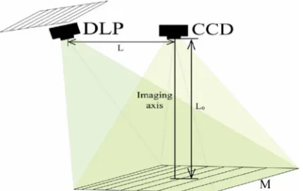
[image:3.612.202.412.182.347.2]3D calibration of a phase calculation-based fringe projection imaging system includes two conversions of phase to depth and pixel to coordinates, called depth calibration and transverse calibration, respectively. Depth calibration builds up the relationship between the absolute phase and the depth data, while transverse calibration establishes the relationship between the pixel positions and the X, Y coordinates. A white plate with a scattered surface was designed and manufactured for 3D calibration. There are 9x12 discrete black hollow ring markers on the surface, as illustrated in Fig. 1. The separation of neighboring markers along row and column direction has the same value of 15 mm with an accuracy of 1 µm.
Fig. 1. A photo image of the manufactured white plate. There are 9x12 black hollow rings on the surface with neighboring separation of 15mm in the horizontal and vertical directions.
Before 3D calibration of the fringe projection system, eight internal parameters of the CCD, including two focal lengths (Fu and Fv), two principal point coordinates (Pu and Pv), and four image radial and tangential distortion coefficients (K1, K2, K3, and K4), need to be determined by capturing the white plate from several random positions. The eight parameters can be calculated from the extracted location of all the hollow ring markers at different plate positions [12,13].
2.1 Marker locations
Fig. 2. Automatically locating the center of all the markers on a captured image of the white plate represented by red dots.
2.2 Depth calibration
Fig. 3. Schematic of even fringe projection at the projector and uneven fringe pattern on the reference M. M: Reference plane.
The fringe pattern has a variable period when projected onto the reference plane due to the crossed optical axes of the imaging and projection devices. This effect is illustrated in Fig. 3 [11]. Therefore, the relationship between absolute phase and depth data is a complicated function of pixel coordinate position of x and y and can be represented by the following equation [4]
( )
(
)
0 2
0
2 0
0 0
,
2 cos cos sin 1
cos sin
, cos sin
L z
L L L
L x
P x y L x
π θ θ θ
θ θ
φ θ θ
=
− +
+
Δ +
(1)
where z is the depth relative to M, Δφ is the difference of the unwrapped absolute phase on the measured object and the plane M, L is the baseline between the CCD camera and the DLP projector, L0 is the working distance to M, θ is the angle between the optical axis of the projector and the camera, and P0 is the period of the projected fringe pattern on a virtual plane perpendicular to the projecting axis. It is difficult and complicated to directly calibrate the systematic parameters of L , L0, θ , and P0 . Here, a polynomial-based calibration method will be used to build up the relationship between absolute phase and depth data.
[image:4.612.200.415.288.424.2]( )
( ) ( )
0
, N n , , n,
n
z x y a x y φ x y
=
=
Δ (2)where a an, n−1,... ,a a2 1 are a coefficient set containing the systematic parameters. Because of the dependence of Eq. (2) on the x and y coordinates, the coefficient set will have different values between pixel positions. Therefore, a Look-Up Table (LUT) needs to be used at each pixel position to build up the relationship between absolute phase and depth data.
Depth calibration means to determine the coefficient set of the polynomial equation which can be realized by placing the white plate at several different positions in the measuring volume. At each position, sinusoidal fringe patterns are projected onto the plate surface to give the absolute phase information of each pixel. The center location [ , ]u v of each marker in the pixel coordinate system is obtained by the marker location method in subsection 2.1. From the obtained center location of each marker, the coordinates of all the markers in the pixel coordinate system at different positions can be determined. The external parameters R
and T of the white plate with regard to the CCD camera are calculated by the following Eq. (3)
[
1]
T[
w w w 1 ,]
Ts u v =A R T x y z (3)
where, R is a matrix representing the three rotation angles, T =[ , , ]T T Tx y z is a vector representing the three linear translations, [ ,x y zw w, ]w is the coordinate vector of a marker P
on the white plate, [ , ]u v is the coordinate vector of P in the pixel coordinate system, A is a matrix of internal parameters of the CCD camera, s is an arbitrary scaling factor and [ ]T
denotes the transposition.
The world coordinate of each pixel point on the white plate is obtained by using the external parameters R and T, so that the relative depth of each pixel to a reference plane is obtained. Therefore, the relationship between absolute phase and depth data at each pixel can be built up by the polynomial Eq. (2) to give accurate depth calibration.
2.3 Transverse calibration
Transverse calibration is to determine the relationship between pixel coordinates and X, Y coordinates. For an actual imaging system, the relationship is nonlinear because of the distortion of optical imaging and projecting lens. Although the MatLab Camera Calibration toolbox can correct for the captured image distortion, there are still some uncorrected distortions from the projecting lens of the DLP projector. Transverse calibration relates to depth information obtained from projected fringe patterns. Therefore, at each pixel position the following two polynomial equations are used to give a high accurate relationship:
2
0 0 0
2
1 1 1
( , ) ( , )
,
( , ) ( , )
r r r
r r r
x a u v z b u v z c
y a u v z b u v z c
= + +
= + +
(4)
where a b c a b c0, , , , ,0 0 1 1 1 are the coefficient set of the system parameters, [ , ]u v is the coordinate vector of a point in the pixel coordinate system, x y zr, ,r r are the coordinates of
the same point on the white plate in the reference coordinate system.
to be established to save the coefficients of each pixel to give a highly accurate relationship between pixel positions and X, Y coordinates.
3. Experiments and results
3.1 Experimental system
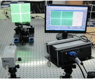
[image:6.612.223.389.272.410.2]The hardware of the fringe projection imaging system includes a portable DLP video projector, a color 3-CCD camera connected to a personal computer (PC) by Firewire IEEE 1394, as illustrated in Fig. 4. The projector is from BenQ (Model CP270) with one-chip digital micro-mirror device (DMD) and a resolution of up to 1024 × 768 pixels (XGA). The colors red, green, and blue are produced by rapidly spinning a color filter wheel in the projector and synchronously modifying the state of the DMD. The 3-CCD camera from Hitachi (Model HV-F22F) has a resolution of 1360 × 1024 pixels. The camera has a standard zoom lens (Computar) with focal length from 12 to 36 mm and adjustable aperture. The personal computer provides system control. The PC graphics card is setup to drive two monitors, one for the DLP and the other for the control software and viewing the captured data. The system can generate red, green, blue or composite color fringe patterns. In the following experiments, green fringe patterns are used to demonstrate the calibration process.
Fig. 4. The hardware setup of the fringe projection imaging system including a DLP projector, a color 3CCD camera and a personal computer.
3.2 3D calibration
A white plate with 9x12 discrete black hollow ring markers was designed and manufactured by Ti-Times [16], as illustrated in Fig. 1. The separation of neighboring markers along the row and column direction has the same value of 15mm. Calibrating the camera parameters needs theoretically at least two captured images from different viewpoints. In order to cover the whole measuring volume and to accurately determine the internal parameters of the CCD camera, the plate was positioned at twenty-four random positions and orientations with a large angle between the imaging axis and the plate’s normal. At each position, the CCD camera captures one image containing all the 9x12 markers. Using the known separation in the twenty-four captured images, the internal parameters of the CCD camera are obtained by the Camera Calibration Toolbox for Matlab [13]. The radial and tangential distortions of the following captured images were corrected by the obtained internal parameters.
marker position determination. Fringes on black hollow rings have low modulation and the absolute phase data for them was interpolated from the surrounding pixels.
In principle, a higher polynomial order can provide more accurate depth data. However, a fifth fitting was found to be sufficient to calibrate the system to the level that could be achieved given the available phase resolution. The coefficient set of the polynomial at one pixel position in Eq. (2) is solved by the absolute phase and depth data. The pixel coordinates and the transverse coordinates on the plate from the thirty-nine images were used to determine the coefficient sets of the other two polynomials by using Eq. (4). All the obtained coefficient sets are saved into three LUTs for late 3D measurement.
[image:7.612.131.467.197.440.2]3.3 Quantitative evaluation
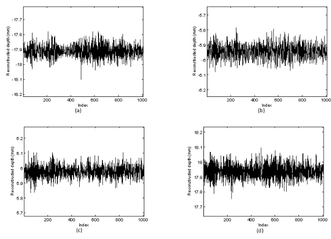
Fig. 5. Measured depth along middle row direction for four positions of −18mm, −6mm, 6mm and 18mm in (a), (b) (c) and (d). X-axis represents the pixel positions along row direction with a range 1,2,3…, 1024, the vertical axis is the reconstructed depth to the reference surface.
In order to evaluate the calibrated fringe projection imaging system, the same plate was placed on an accurate translating stage with resolution of 1μm. The plate was positioned at
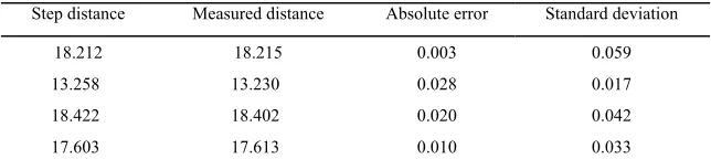
−18mm, 6mm, −6mm and −18mm with respect to the reference plane M. At each position, the depth data was calculated using the obtained coefficient sets from Eq. (2). The profile along one row near the middle is illustrated in Fig. 5 for the four positions. The measured average value, absolute error (absolute difference between the measured average distance and the distance by the stage) and standard deviation value along the middle row for the four positions were listed in the 4th, 7th and 10th column in Table 1, respectively.
Table 1. Experimental results on the accurately positioned plate at-18mm, 6mm, −6mm and −18mm (Unit: mm)
Position Measured distance Absolute error Standard deviation
X Y Z X Y Z X Y Z
−18 14.966 14.966 −17.913 0.034 0.034 0.087 0.029 0.029 0.042
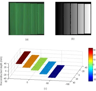
[image:7.612.110.502.607.667.2]Fig. 6. Illustration of the step artifact and the measured 3D shape data. (a) the step artifact with green projected fringe, (b) absolute phase map, and (c) the measured 3D shape.
By utilizing the obtained coefficient sets from Eq. (4) and the depth value at each plate position, the transverse X, Y coordinates of all the ring markers on the white plate can be calculated, so the measured distance between neighboring ring markers is obtained. Table 1 lists the average distance between all the markers along the X and Y direction in the 2nd and 3rd column respectively. The absolute error between the measured distance and 15mm is listed in in the 5th and 6th column respectively. The 8th and 9th column show the standard deviation of the measured distance along the X and Y direction. The experimental results on the four plate positions show that the proposed 3D calibration method accurately converts not only absolute phase into depth data but also pixel positions into transverse X and Y coordinates.
results show again the proposed 3D calibration method accurately converts absolute phase into depth data.
Table 2. The experimental results on the measured step (Unit: mm) Step distance Measured distance Absolute error Standard deviation
18.212 18.215 0.003 0.059 13.258 13.230 0.028 0.017
18.422 18.402 0.020 0.042 17.603 17.613 0.010 0.033
3.4 Qualitative evaluation
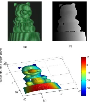
A toy having freeform surface was measured by the calibrated fringe projection imaging system. Twelve sinusoidal fringe patterns having the optimum fringe numbers of 100, 99 and 90 [17] were projected via green channel onto the toy’s surface for absolute phase calculation. Figure 7(a) shows one of the captured fringe pattern image. Figure 7(b) illustrates the absolute phase map obtained by using optimum three fringe number selection method. During the process of phase calculation, pixels with a modulation less than 15 grayscales are marked as invalid and these pixels are shown in black. The 3D shape data of the toy were obtained after converting the absolute phase map into depth and transverse data, as shown in Fig. 7(c).
4. Conclusions
As proposed, a simple, flexible and automatic 3D calibration method was developed for a phase calculation-based fringe projection imaging system. A white plate was used whose surface was marked with discrete hollow ring with a known separation. By placing the plate at several random positions, the internal parameters of the CCD camera can be determined. The plate also can give absolute phase and depth data in the measuring volume to build up their relationship by a polynomial function at each pixel position. At each plate position, the absolute phase of each pixel can be calculated by projecting three fringe pattern sets with the optimum fringe numbers onto the plate surface. From the captured images, the location of all the markers is automatically and accurately extracted without any manual operation, so the relative depth of each pixel to a chosen reference plane can be obtained. Therefore, the coefficient set of the polynomial function are calculated by using the obtained absolute phase and depth data. The pixel positions and X, Y coordinates can be established by the parameters of the CCD camera and the obtained depth data. Four known depths of the plate and a ‘step artifact’ have been tested and the experimental results show the validity and flexibility of the proposed 3D calibration method. Therefore, the proposed method has the potential for accurate 3D calibration of phase calculation-based fringe projection imaging system with minimal operator skill and in a robust, flexible and automatic manner.
Fig. 7. The measured results on a toy having freeform surface. (a) photo of the toy with green projected fringe, (b) absolute phase map, and (c) the measured 3D shape.
Acknowledgments