Moamar, Hamed, Tesfa, Belachew, Fengshou, Gu and Ball, Andrew
Vehicle Suspension Performance Analysis Based on Full Vehicle Model for Condition Monitoring
Development
Original Citation
Moamar, Hamed, Tesfa, Belachew, Fengshou, Gu and Ball, Andrew (2014) Vehicle Suspension
Performance Analysis Based on Full Vehicle Model for Condition Monitoring Development. In:
VETOMACX 2014, 911th September 2014, University of Manchester, UK. (Unpublished)
This version is available at http://eprints.hud.ac.uk/id/eprint/20452/
The University Repository is a digital collection of the research output of the
University, available on Open Access. Copyright and Moral Rights for the items
on this site are retained by the individual author and/or other copyright owners.
Users may access full items free of charge; copies of full text items generally
can be reproduced, displayed or performed and given to third parties in any
format or medium for personal research or study, educational or notforprofit
purposes without prior permission or charge, provided:
•
The authors, title and full bibliographic details is credited in any copy;
•
A hyperlink and/or URL is included for the original metadata page; and
•
The content is not changed in any way.
For more information, including our policy and submission procedure, please
contact the Repository Team at: E.mailbox@hud.ac.uk.
Vehicle Suspension Performance Analysis Based
on Full Vehicle Model for Condition Monitoring
Development
Moamar. Hamed, Belachew. Tesfa, Fengshou. Gu and Andrew. D. Ball
Centre for Efficiency and Performance Engineering, University of Huddersfield, Huddersfield, HD1 3DH, UK
Email: U0951001@hud.ac.uk
Abstract The objective of this research is to develop a mathematical model
us-ing a seven degree-of-freedom full car. The simulation analyses were conducted to predict the response of the vehicle when driven across speed bumps of different shapes and at range of speeds. Three bump sizes were considered in this study in-cluding bump 1 (500 mm x 50 mm), bump 2 (500 mm x 70 mm), and bump 3 (500 mm x 100 mm). These were run through the model at speeds of 8 km/hr, 16 km/hr, 24 km/hr and 32 km/hr. The model was validated using experimental data, which was collected by driving the vehicle across the bump 1 at a speed of 8km/h. The performance of the suspension in terms of ride comfort, road handling and stability of the vehicle were analysed and presented. The vibration analysis for dif-ferent speed levels of 8 km/hr, 16 km/hr, 24 km/hr and 32 km/hr indicated that, the effect of vehicle speeds on the vibration of the vehicle body increases at lower speeds up to a maximum value after which it began to decrease from the optimum point with increasing vehicle speeds. The model has been used for fault detection of under-inflation of vehicle tyre by 35%, and also to predict possible future sus-pension faults.
Key words Condition monitoring, suspension modeling, vibration measurement,
speed bump geometry, vehicle speed.
1.0 Introduction
Suspension systems and their components have significant influence on passenger safety, ride comfort, handling, and vehicle stability. According to the
Ministry of
%) attributed for a high number of re-tests followed by suspension faults (13.18 %), brake faults (11.47 %) and tyre faults (8.75 %). As shown in the pie chart (Figure 1), suspension and tyres faults are the 2nd and the 4rt frequent faults in MOT tests respectively. To consider the performances of the suspension in terms of ride quality, handling and stability of the vehicle, some important parameters must be studied; these parameters are the wheel deflection, suspension travel and the vehicle body acceleration.
Fig. 1 Percentage of failure by category for different cars
The aim is to achieve small amplitude value for these parameters [2]. Road han-dling is associated with the relative displacement between suspension and the road input (Zu - Zr). This is represented as wheel deflection as shown in the Figure 2. Suspension travel is defined as the relative vertical displacement between the ve-hicle body and the wheel (Zs – Zu) as shown in the Figure 2. This can be used for assessing the space required to accommodate the suspension spring. Ride comfort is related to vehicle body motion sensed by the passenger’s comfort. This requires that the acceleration of the vehicle body (sprung mass) be relatively small. Ac-cording to ISO: 2631-1-1997 [3] the proper road handling must be in the range of 0.0508 m whilst the standard value for suspension travel must be in the range of minimum of 0.127 m. Finally, the passenger feels highly comfortable if the RMS acceleration is below 0.315 m/s2.
ks cs
mu kt
ms
zr ZS
zu ZS – Zu
Zu – Zr ct
Fig. 2 Sketch of quarter car model
A number of researchers have investigated suspension performance using model-ling/simulation [4]. A mathematical model for quarter car with 2-DOF and a half
19.79
13.18
8.75 11.47 8.23 5.82 3.55
1.11 1.72 1.32 0.46 Lighting and signalling Suspension
Tyres Brakes
Driver's view of the road Fuel and exhaust Steering
Registration plates and VIN Seat belts
[image:3.595.142.462.244.349.2]3
car with 4-DOF have been investigated by Faheem [5]. Also, a mathematical model of a 3-DOF quarter car with semi-active suspension system has been devel-oped by Rao [6]. The model was used for testing of skyhook and other strategies of semi active suspension system. Modeling of one and two DOF for a quarter car design asemi-active twin-tube shock has been developed by Esslaminasa et al.[7]. Darus [8] adopted a state space approach in developing a mathematical model for both a quarter car and full car using MATLAB packages. In Metallidis [9], statis-tical system identification technique was applied for performing parametric identi-fication and fault detection of nonlinear vehicle suspension system. A model-based fault detection applied on a vehicle control system has been presented by Kashi [10], which relies on mathematical descriptions of the system and which yields a robust fault detection and isolation of faults affecting the system. Agharkakli et al. [11] presents a mathematical model for passive and active of quarter car suspension system. A research study to improve road handling and rid comfort was presented by Ikenaga et al. [12]. Active suspension control system based on a full Vehicle model was presented, and the performance of suspension system was included. The effect of truck speed on the shock and vibration levels was discussed by Lu et al [13]. They indicated that the effect of truck speed on root mean square acceleration of vibration was strong at a lower speed, but slight at a higher speed.
The objective of this research is to analyse the performances of suspension in terms of ride comfort, road handling and stability. The effect of road conditions, vehicle speed and any changing in suspension specifications include the effect of tyre pressure, have been investigated. For this a mathematical modelling of the full car has been conducted in this study.
To develop the vehicle model, it can be assumed that the vehicle is a rigid body and represented as sprung mass ms, while suspension axles represented as
un-sprang mass mu as shown in Figure 3. The suspension between the vehicle body
and wheels are modelled by simple linear spring and damper elements, and also each tyre is modelled as a single linear spring and damper.
ms
mu mu mu
mu L2
L1
Pitch axis
wf/2 wf/2
ktf ktr
zr2 z
r1
zr4
zr3
zu1
zu2
zu3
zu4
kf Cf kr
Cf Cr
Roll axis
kf
kr Cr
wr/2 wr/2
Ctr ktr Ctr ktf Ctf
Ctf
zs
[image:4.595.135.414.541.653.2]the equations of all motions are derived separately, and finally the equations of the body motions are achieved [8].
Equation of motion for bouncing of sprung mass:
̈
(
)
(
)
(
)
(
)
( ̇
̇
)
( ̇
̇
)
( ̇
̇
)
( ̇
̇
)
(1)
For pitching moment of inertia of sprung mass
̈
(
)
(
)
(
)
(
)
( ̇
̇
)
( ̇
̇
)
( ̇
̇
)
( ̇
̇
)
(2)
For rolling motion of the sprung mass
̈
(
)
(
)
(
)
(
)
( ̇
̇
)
( ̇
̇
)
( ̇
̇
)
( ̇
̇
)
(3)
For each wheel motion in vertical direction
̈
(
)
( ̇
̇
)
(
)
( ̇
̇
)
(4)
̈
(
)
( ̇
̇
)
(
)
( ̇
̇
)
(5)
̈
(
)
( ̇
̇
)
(
)
( ̇
̇
)
(6)
̈
(
)
( ̇
̇
)
(
)
( ̇
̇
)
(7)
5
The road profile is assumed to be a single bump with sin wave shape; it was calcu-lated and created according to vehicle speeds, height and width of the bumps by the following equation:
( ) ( )
(8) [image:6.595.132.465.331.533.2]Where (a) is the bump height, which was considered in this study as [50, 70 and 100 mm], frequency of the bump which was calculated by considering length of the bump and vehicle speed, t is the time for crossing the vehicle on the bump. Three bump sizes were considered in this study such as: bump 1 (500 mm in width x 50 mm height), bump 2 (500 mm in width x 70 mm height), and bump 3 (500 mm in width x 100 mm height). The models were simulated for speeds of 8 km/hr, 16 km/hr, 24 km/hr and 32 km/hr for validations.
Table 1 Shows definition of equations variables and parameters of suspension
Variables Definitions Units
= 1290 Sprung mass (mass of the body) Kg
, = 85 Unsprang mass Kg
Roll and pitch of moment of inertia Kg m² Distance from front and rear wheel
to the car centre
m
Stiffness of front and rear spring N/m
Stiffness of front and rear tyre N/m
Front and rear damper coefficient
for
Nm/sec
Front and rear vehicle width m
Displacement of the vehicle body m
θ, φ Roll and pitch angles rad
2.0 Experimental set up and test procedures
In order to insure significant installation for the sensors, two different adapters were designed and manufactured at the University of Huddersfield. In addition, a wireless measurement system was also designed and installed on the car to offer a complete remote measurement for vibration and pressure data. The two sensors were connected to the wireless sensor nodes (transmitters) assembled and situated in the centre rim of the front left wheel for the pressure sensor, and inside the car for the vibration sensor. The gateway (receiver) was equipped together with a lap-top inside the car.
The main aim of this test was to obtain the acceleration (vibration) response of the suspension system in order to analyze the effect of velocity change and under-inflation of the tyre on the performance of the suspension system. The test was conducted with standard tyre pressure (2.3bar) and vehicle speed of 8km/h.
3.0 Results and Discussion
The model was validated using experimental data collected by driving the vehicle across the bump1 (located in the University of Huddersfield premises) with speed of 8 km/h.
Fig. 4 Vibration (acceleration) of suspension simulation and experimental
The bump profile used was 5.80 m width, 0.50 m length and 0.050 m height. The MATLAB software was used to analyse the response of the vehicle. Figure 4 de-picts the acceleration of vehicle body in time domain based on model simulation and experiments. It can be noted that the model fairly predicts the performance of the suspension in comparison with the experimental results. The plots of the road profile for the three bumps in time domain are shown in the Figure 5-a, for front and rear wheel of the vehicle.
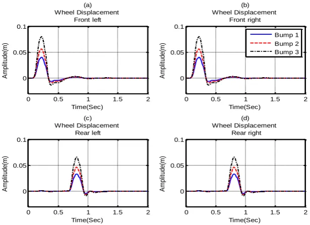
For the simulation study, road disturbance is assumed as the input for the system. Figure 5-b shows the displacement of the vehicle body (sprung mass) while Figure 6 shows the displacement of four wheels (unsprung mass) in time domain. From
0 0.2 0.4 0.6 0.8 1 1.2 1.4 1.6 1.8 2
-5 0 5
Time(Sec)
A
c
c
e
le
ra
ti
o
n
(
m
/s
2) Simulation
[image:7.595.137.451.404.523.2]7
these plots, it can be seen that the amplitude of the vehicle body and the wheels increase stably with increase in the bump height. This indicates that the perfor-mance of the suspension may be affected by this change in the geometry of bumps or road disturbances.
Fig. 5 (a) Road profile excitation and (b) displacement of vehicle body for different road bumps
Fig. 6 Vehicle wheel’s displacement with different road profile (bumps)
0 0.2 0.4 0.6 0.8 1 1.2 1.4 1.6 1.8 2
0 0.05 0.1 Time(Sec) H ( m )
(a) Road Profile Exitation
Bump 3
0 0.2 0.4 0.6 0.8 1 1.2 1.4 1.6 1.8 2
-0.02 0 0.02 0.04 0.06
(b) Car Body Displacement
Time(Sec) A m pl itu de (m ) Bump 1 Bumpp 2 Bump 3
0 0.5 1 1.5 2
0 0.05 0.1 (a) Wheel Displacement Front left Time(Sec) A m pl itu de (m )
0 0.5 1 1.5 2
0 0.05 0.1 (b) Wheel Displacement Front right Time(Sec) A m pl itu de (m )
0 0.5 1 1.5 2
0 0.05 0.1 (c) Wheel Displacement Rear left Time(Sec) A m pl itu de (m )
0 0.5 1 1.5 2
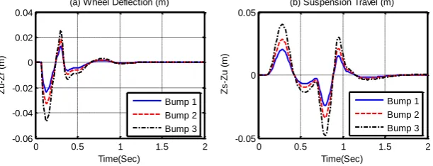
[image:8.595.129.416.198.371.2] [image:8.595.130.438.405.628.2]To analyse the performances of the suspension in terms of ride quality, handling and stability of the vehicle, road handling profile for vehicle is associated with the contact forces between the road surface and the vehicle tyre (zu – zr). The wheel deflection for this simulation was about 0.011 m, 0.015 m and 0.025 m for bump1, bump 2 and bump 3 respectively as presented in Figure 7-a. This range of wheel deflection seems to be acceptable compared with the proper road handling which must be in the range of 0.0508 m as per ISO: 2631-1-1997 [3].
Fig. 7 (a) Wheel deflections and (b) suspension travel for different bumps
The suspension travel can be defined as a relative displacement between the vehi-cle body and the wheel (zs – zu) as shown in Figure 7-b. The value is about 0.02 m, 0.028 m and 0.04 m for passing the vehicle over bump1, bump 2 and bump 3 respectively. This range of suspension travel seems to be acceptable in comparison with the standard value which must have a minimum value of 0.127m according to the ISO: 2631-1-1997 specification [3]. In addition, ISO: 2631-1-1997 [3] also states that, the passenger feels highly comfortable if the RMS acceleration is be-low 0.315 m/s2. In Figure 8, the acceleration of the vehicle body in time domain is presented. The results agree with both the ISO specification and with results pre-sented in previous researches [11]. Figure 9 shows a typical example of RMS val-ue for acceleration of the vehicle body at different speed levels of 8 km/hr, 11 km/hr, 16 km/hr, 24 km/hr and 32 km/hr, and with different bump sizes. These re-sults show that the effect of vehicle speed on the acceleration of the vehicle body is strong at lower speeds and slight at high speeds. It can be clearly noted that, the change of the RMS value was high with changing speeds at values between 8 to 11 km/hr compared to changing the speed at high values between 11 to 16km/hr. It should also be noted that, the highest acceleration occurs during the speed of 11–16 km/hr. These results have been compared with [13] and show some agree-ment.
The transfer function was used to detect the level of under-inflation of the tyre and also predict possible future suspension faults. In Figure 10, the amplitude-frequency characteristic curves for changes of tyre stiffness in four different out-put cases (vehicle body vertical displacement, vehicle body velocity, displacement of front wheel, and displacement of rear wheel) are shown. . From the plots, it can
0 0.5 1 1.5 2
-0.06 -0.04 -0.02 0 0.02 0.04
(a) Wheel Deflection (m)
Time(Sec)
Z
u
-Z
r
(m
)
Bump 1 Bump 2 Bump 3
0 0.5 1 1.5 2
-0.05 0 0.05
(b) Suspension Travel (m)
Time(Sec)
Z
s
-Z
u
(
m
)
9
[image:10.595.134.415.220.571.2]be seen that every vibration response value causes resonance phenomenon and generates peak values in the vicinity of about 1 Hz and 9 Hz. The vibration re-sponse value becomes larger in resonance region as the decrease of tyre stiffness. In the high frequency resonance region, there is a change in the vibration response values which is related to the wheels however the vibration response values relat-ed to the vehicle’s body shows also high change.
Fig. 10 Transfer function response for vehicle body and vehicle body velocity
4.0 Conclusion
A 7-DOF model for a full vehicle has been developed to analyse the time and the frequency response of the vehicle in MATLAB. The performances of the
suspen-0 0.2 0.4 0.6 0.8 1 1.2 1.4 1.6 1.8 2
-8 -6 -4 -2 0 2 4 6 Time(Sec) A c c e le ra ti o n ( m /s 2)
Car Body Vibration
Bump 1
Bump 2 Bump 3
Bump (0.05m) Bump (0.07m) Bump(0.1m)
0.5 1 1.5 2 2.5 3 Bump A m p lit u d e ( m /s e c 2)
RMS of vehicle body acceleration
V= 8 Km/hr
V= 11 Km/hr
V= 16 Km/hr V= 24 Km/hr V= 32 Km/hr
101 -40 -30 -20 -10 0
From: d11 To: vdb
M a g n itu d e ( d B )
Response to road input f or body displecement
Frequency (rad/sec) 2.3 bar Passenger 1.5 bar Driver 1.5 bar Both 1.5 bar
101 0 5 10 15 20 25 30
From: d11 To: vb
M a g n itu d e ( d B )
Response to road input f or body velocity
Frequency (rad/sec)
101 -10 -5 0 5 10
From: d11 To: df rw
M a g n itu d e ( d B )
Response to road input f or f ront w heel
Frequency (rad/sec)
2.3 bar Passenger 1.5 bar Driver 1.5 bar Both 1.5 bar
101 -40 -35 -30 -25 -20 -15 -10
From: d11 To: drrw
M a g n itu d e ( d B )
Response to road input f or rear w heel
Frequency (rad/sec)
2.3 bar Passenger 1.5 bar Driver 1.5 bar Both 1.5 bar Fig. 8 Shows acceleration of the
ve-hicle body with different bump sizes
[image:10.595.135.426.224.347.2] [image:10.595.142.401.386.575.2]sion in terms of ride comfort, road handling and stability of the vehicle were pre-sented. The acceleration analysis of the vehicle body for different speed levels of 8 km/hr, 16 km/hr, 24 km/hr and 32 km/hr showed that the effect of vehicle speed on the acceleration of the vehicle body was higher at a low speed and reduced uni-formly at higher speeds. Moreover, the influence of parameter variations on trans-fer functions as a method of fault detection of suspension has been introduced. This approach has been used for fault detection of under-inflation of tyre for three conditions.
References
[1] H. John, “Good Garages | Honest John.” [Online]. Available: http://good-garage-guide.honestjohn.co.uk/.
[2] B. L. Zohir, “Ride Comfort Assessment in Off Road Vehicles using passive and semi-active suspension.”
[3] A. Mitra, N. Benerjee, H. Khalane, M. Sonawane, D. JoshI, and G. Bagul, “Simulation and Analysis of Full Car Model for various Road profile on a analytically validated MATLAB/SIMULINK model,” IOSR J. Mech. Civ. Eng. IOSR-JMCE, pp. 22–33.
[4] G. Verros, S. Natsiavas, and C. Papadimitriou, “Design Optimization of Quarter-car Models with Passive and Semi-active Suspensions under Random Road Excitation,” J. Vib. Control, vol. 11, no. 5, pp. 581–606, May 2005.
[5] F. Alam, A. Faheem, R. Jazar, and L. V. Smith, “A Study of Vehicle Ride Performance Us-ing a Quarter Car Model and Half Car Model,” pp. 337–341, Jan. 2010.
[6] R. Rao, T. Ram, k Rao, and P. Rao, “Analysis of passive and semi active controlled suspen-sion systems for ride comfort in an omnibus passing over a speed bump,” Oct-2010. [7] N. Eslaminasab, M. Biglarbegian, W. W. Melek, and M. F. Golnaraghi, “A neural network
based fuzzy control approach to improve ride comfort and road handling of heavy vehicles using semi-active dampers,” Int. J. Heavy Veh. Syst., vol. 14, no. 2, pp. 135–157, Jan. 2007. [8] R. Darus and Y. M. Sam, “Modeling and control active suspension system for a full car
mod-el,” in 5th International Colloquium on Signal Processing Its Applications, 2009. CSPA 2009, 2009, pp. 13–18.
[9] P. Metallidis, G. Verros, S. Natsiavas, and C. Papadimitriou, “Fault Detection and Optimal Sensor Location in Vehicle Suspensions,” J. Vib. Control, vol. 9, no. 3–4, pp. 337–359. 2003. [10] K. Kashi, D. Nissing, D. Kesselgruber, and D. Soffker, “Diagnosis of active dynamic con-trol systems using virtual sensors and observers,” in 2006 IEEE International Conference on Mechatronics, 2006, pp. 113–118.
[11] A. Agharkakli, G. Sabet, and A. Barouz, “Simulation and Analysis of Passive and Active Suspension System Using Quarter Car Model for Different Road Profile,” Int. J. Eng. Trends Technol.-, vol. 3, no. 5, 2012.
[12] S. Ikenaga, F. L. Lewis, J. Campos, and L. Davis, “Active suspension control of ground ve-hicle based on a full-veve-hicle model,” in American Control Conference, 2000. Proceedings of the 2000, 2000, vol. 6, pp. 4019–4024 vol.6.