Essays in financial economics

Science

Essays in Financial Economics

Olga A. Obizhaeva

Thesis submitted to the Department of Finance of the London

School of Economics and Political Science for the degree of

Doctor of Philosophy

I certify that the thesis I have presented for examination for the PhD degree of the London School of Economics and Political Science is solely my own work other than where I have clearly indicated that it is the work of others (in which case the extent of any work carried out jointly by me and any other person is clearly identified in it).

The copyright of this thesis rests with the author. Quotation from it is permitted, provided that full acknowledgement is made. This thesis may not be reproduced without my prior written consent.

I warrant that this authorisation does not, to the best of my belief, infringe the rights of any third party.

Statement of conjoint work

I confirm that chapter 2 is jointly co-authored with Albert S. Kyle and Anna A. Obizhaeva. Albert S. Kyle has worked as a consultant for various companies, ex-changes, and government agencies. He is a non-executive director of a U.S.-based asset management company. I contributed 33% of the work for chapter 2.

Acknowledgement

I would like to thank my supervisors Dong Lou and Igor Makarov for their guid-ance and support. I am grateful to Amil Dasgupta and Ulf Axelson for supervision in my early years at LSE. I benefited from discussions with the faculty of Finance department at LSE. I would also like to acknowledge the financial support from the London School of Economics and the Systemic Risk Centre. I would not be where I am now without support of Pete Kyle, Mark Kritzman, and Anna Obizhaeva who have been inspiring examples of researchers.

The five years at LSE were very special thanks to my cohort: Jesus Gorrin, Michael Punz, Una Savic, and Seyed Seyedan. We outstay the hurrying flight of years, bear-ing with each other through laughter and through tears. I have been lucky to be surrounded by my fellow PhD students: Lorenzo Bretscher, Svetlana Bryzgalova, Fabrizio Core, Sergei Glebkin, Inna Grinis, James Guo, Andrea Englezu, Lukas Kre-mens, John Kuong, Dimitris Papadimitriou, Paola Pederzoli, Bernardo Ricca, Gosia Ryduchowska, Petar Sabtchevsky, Su Wang, Yue Yuan, Zizi Zeng.

This thesis consists of three essays in financial economics.

The first chapter analyses the fundraising process in the hedge fund industry and the role financial intermediaries play in this process. Using the SEC form D filings, I document that broker-sold funds underperform directly-sold funds by 2% (1.6%) per year on a risk-adjusted basis before (after) fees. Also directly-sold funds, on average, have larger average investor’s size, larger minimum investment size, and charge higher performance fees comparing to broker-sold ones. Empirical results are consistent with a stylized model of fundraising. I estimate the model implied average broker’s compensation to be $1.5 million per year.

The second chapter (co-authored with Albert S. Kyle and Anna A. Obizhaeva) introduces a new structural model of stock returns generating process. The model assumes that stock prices change in response to buy and sell bets arriving to the market place as predicted by market microstructure invariance. These bets are shredded by traders into sequences of transactions according to some bet-shredding algorithms. Arbitrageurs take advantage of any noticeable returns predictability, and market makers clear the market. This structural model is calibrated to match empirical time-series and cross-sectional patterns of higher moments of returns. We calibrate hard-to-observe parameters of bet-shredding using the method of simulated moments, analyse its properties, and show how much shredding has increased over time.

1 Fundraising in the Hedge Fund Industry 9

1.1 Data . . . 15

1.1.1 Form D filings . . . 15

1.1.2 Morningstar database and risk-adjusted returns . . . 18

1.1.3 Matching form D filings and Morningstar database . . . 22

1.2 Empirical evidence . . . 24

1.2.1 After-fee performance across distribution channels . . . 25

1.2.2 Pre-fee performance across distribution channels . . . 28

1.2.3 Fees across distribution channels . . . 30

1.2.4 Clientele across distribution channels . . . 31

1.3 Theoretical motivation . . . 32

1.3.1 Model of fundraising . . . 32

1.3.2 Model implications . . . 43

1.3.3 Compensation for the broker . . . 45

1.4 Conclusion . . . 46

1.5 Tables and figures . . . 48

1.6 Capital inflows estimation . . . 66

1.7 Robustness checks . . . 68

2 Order Shredding, Invariance, and Stock Returns 75 2.1 Introduction . . . 75

2.2 Moments of daily returns: empirical analysis . . . 78

2.2.1 Data . . . 78

2.2.3 Time-series and cross-section of empirical moments . . . 82

2.3 Invariance-implied structural model of price dynamics . . . 84

2.3.1 Bets of traders . . . 84

2.3.2 Price changes upon execution of one bet . . . 86

2.3.3 Price changes upon execution of bet sequences with no bet shredding . . . 87

2.3.4 Price changes upon execution of bet sequences with no bet shredding . . . 88

2.3.5 Price changes upon execution of bet sequences with bet shred-ding . . . 90

2.3.6 Price dynamics with shredding and arbitrageurs . . . 94

2.3.7 Properties of simulated returns . . . 96

2.4 Properties of implied shredding parameter . . . 98

2.5 Conclusions . . . 100

2.6 Tables and figures . . . 102

3 Size of Share Repurchases and Market Microstructure 120 3.1 Introduction . . . 120

3.2 Share repurchases and invariance . . . 123

3.2.1 Review of market microstructure invariance . . . 123

3.2.2 Share repurchases hypotheses . . . 124

3.2.3 Nested models . . . 129

3.3 Data . . . 130

3.4 Results . . . 134

3.4.1 Hypothesis testing . . . 134

3.4.2 Model selection . . . 137

3.4.3 Alternative hypotheses . . . 138

3.5 Conclusion . . . 140

1.1 Outline of form D filings . . . 49

1.2 Largest funds by distribution channel . . . 50

1.3 Top players in fundraising industry . . . 51

1.4 Summary statistics . . . 53

1.5 After-fee systematic risk exposure of hedge funds . . . 55

1.6 Pre-fee systematic risk exposure of hedge funds . . . 56

1.7 Alphas of directly and broker sold hedge funds . . . 59

1.8 Value added by directly and broker sold hedge funds . . . 60

1.9 Heterogeneity of brokers . . . 61

1.10 Heterogeneity of brokers . . . 62

1.11 Fees of directly sold and broker sold funds . . . 63

1.12 Clientele of directly sold and broker sold funds . . . 64

1.13 Average broker fee: bargaining power . . . 65

1.14 Performance of Hedge Fund Portfolios: After Fee + Bias . . . 69

1.15 Performance of hedge fund portfolios: pre fee + bias . . . 70

1.16 Alphas of directly and broker sold hedge funds . . . 71

1.17 Value added by directly and broker sold hedge funds . . . 72

1.18 Heterogeneity of brokers . . . 73

1.19 Heterogeneity of brokers . . . 74

2.1 Kurtosis and skewness for trading activity groups across decades . . . 109

2.2 Simulated theoretical kurtosis and low bounds. . . 110

2.3 Imbalance forecasting model of arbitrageurs. . . 111

2.5 Summary statistics for daily returns. . . 117

2.6 Calibrated bet-shredding parameters. . . 118

2.7 Implied execution horizons. . . 119

3.1 Hypotheses predictions . . . 130

3.2 Descriptive statistics. . . 143

3.3 Descriptive statistics by repurchase method. . . 144

3.4 Size of repurchase program and trading activity. . . 146

3.5 Size of repurchase program and trading activity. . . 147

3.6 Nested regression. . . 149

3.7 Nested regression across repurchase types. . . 150

3.8 Model selection. . . 151

1.1 Time line of the fundraising game . . . 34

1.2 Separating equilibria of the fundraising game . . . 37

1.3 Fundraising in alternative investment industry . . . 52

1.4 Performance of directly sold and broker sold hedge funds . . . 54

1.5 After-fee alphas of directly sold and broker sold hedge funds . . . 57

1.6 Pre-fee alphas of directly sold and broker sold hedge funds . . . 58

1.7 Performance of hedge fund portfolios: after fee + no bias correction . 68 2.1 Idiosyncratic kurtosis of daily stock returns for 1950 through 2016. . . 103

2.2 Ratio of idiosyncratic kurtosis (Group 1 to Group 10) for 1950 through 2016. . . 104

2.3 Kurtosis of daily stock returns for 1950 through 2016. . . 105

2.4 Ratio of kurtosis (Group 1 to Group 10) for 1950 through 2016. . . . 106

2.5 Idiosyncratic skewness of daily stock returns for 1950 through 2016. . 107

2.6 Idiosyncratic volatility of daily stock returns for 1950 through 2016. . 108

2.7 Returns autocorrelations without arbitrager. . . 112

2.8 Returns autocorrelations with arbitrager. . . 113

2.9 Distributions of simulated moments without arbitrageurs . . . 115

2.10 Distributions of simulated moments with arbitrageurs . . . 116

3.1 Historical share repurchase activity. . . 142

3.2 Sizes of share repurchase programs versus trading activity of stocks . 145 3.3 Size of repurchase program and trading activity (yearly). . . 148

Fundraising in the Hedge Fund

Industry

High search and due diligence costs due to the opacity of the hedge fund industry make the fundraising process challenging even for hedge funds with a good reputa-tion and a strong track record. Financial intermediaries, such as brokers, consul-tants, and placement agents, help funds and investors to find one another and to overcome barriers to transact. This paper studies, empirically and theoretically, the role of intermediaries in the fundraising process of hedge funds.

There is yet no consensus about the role and social value of intermediaries. Some people think that intermediation is socially useful. This view is usually justified with several arguments. First, intermediaries may help counterparties find one another and transact, by exploiting their positional advantage and industry knowledge, as per Rubinstein and Wolinsky (1987). Second, intermediaries may help alleviate adverse selection problems, as per Booth and Smith (1986) and Garella (1989). Third, intermediaries may add value by decreasing the costs of making decisions and executions, as per Spulber (2001).

Others think that intermediaries impose unnecessary costs on society. Judge (2014) argues that intermediaries often promote institutional arrangements to max-imize their economic rents, and illustrates her point using examples of real estate agents, stock brokers, mutual funds, and exchanges. Warren Buffett opposed and

publicly criticized intermediaries on numerous occasions. For example, in 1996 class B shares of Berkshire Hathaway were issued as a response to unit trusts that sold fractional units of Berkshire’s shares to small investors.

To analyze empirically the role that financial intermediaries play in the fundrais-ing process of hedge funds, I download and process the entire collection of form D filings that hedge funds report to the U.S. Securities and Exchange Commission (“the SEC”) under Regulation D. These filings have information on all third parties involved in the fundraising process. It allows one to identify the hedge funds offered to investors directly and those sold to investors through intermediary brokers.

I match this dataset with the Morningstar hedge funds database using a fuzzy match algorithm. My final dataset combines information on fundraising process, contract characteristics, and performance of hedge funds.

First, I find that, on average, broker-sold funds underperform the directly-sold funds by a substantial margin. Following Fung and Hsieh (2004), I find that broker-sold funds again consistently underperform directly-broker-sold funds by 1.6% on a risk-adjusted basis after accounting for fees. As suggested by Berk and van Binsbergen (2013), the measure of the dollar value added of broker-sold funds is, on average, $210,000 per month lower than that of directly-sold funds.

Second, I construct gross returns series using the modified methodology de-veloped by Brooks, Clare and Motson (2007), Hodder, Jackwerth and Kolokolova (2012), and Kolokolova (2010), and document that broker-sold funds underperform directly-sold funds by 2% per year before fees as well. The pre-fee dollar value added by broker-sold funds is, on average, $190,000 per month lower than that of directly-sold funds. Since pre-fee risk-adjusted performance is a likely indication of skill, this evidence contradicts the view that intermediaries help to identify skillful funds.

Third, I find that, on average, funds sold by brokers charge lower incentive fees compared to funds sold directly, whereas there is no significant difference in terms of management fees.

in-for the accredited investor status based on their income or net worth, suggesting that size is correlated with sophistication of investor. Therefore, this evidence im-plies that broker-sold funds and directly-sold funds may target different clienteles; directly-sold funds attract, on average, more sophisticated investors than broker-sold funds.

Finally, I analyze heterogeneity of brokers, classifying brokers into in-house and outside brokers based on the similarity of names of a fund and a broker. I find that funds sold by in-house brokers underperform directly-sold funds by 2.1% per year on a risk-adjusted basis after accounting for fees, while funds sold by outside brokers underperform directly-sold funds by 1.4% per year. Funds sold by in-house and outside brokers underperform directly-sold funds by 2% per year on a risk-adjusted basis before accounting for fees. Moreover, funds sold by outside brokers have lower incentive fees than funds sold directly, while the incentive fees of funds sold by in-house brokers do not differ from those of funds sold directly. Funds that are sold through outside brokers have a lower minimum investment sizes than that of directly-sold funds, while the minimum investment sizes of funds sold through in-house brokers do not differ from that of directly-sold funds.

The choice of fundraising channels is an equilibrium outcome; therefore these empirical findings have no causal interpretation, but rather provide an empirical description of an equilibrium. I present a stylized theoretical model of fundraising in the hedge fund industry and show that the implications of the model are consistent with documented empirical findings. The model builds on the work of Nanda, Narayanan and Warther (2000) and Stoughton, Wu and Zechner (2011).

Sophisticated investors have low search and due diligence costs, others have no industry connections and face high search and due diligence costs. I solve for a separating equilibrium, in which funds endogenously choose portfolio management fees and capital-raising channels, whereas investors decide to invest into hedge funds on their own or based on recommendation of an intermediary.

This equilibrium has a simple intuition. The existence of both types of funds is socially optimal, since both funds generate positive returns, which are greater than the outside option. Some investors, however, are not able to invest in the hedge fund industry without financial advice. Only sophisticated investors can find the good fund, while other investors with high due-diligence costs are not able to do so. The broker steps in to resolve this inefficiency. The broker is able to lower the costs of investors by internalizing the due-diligence process and this allows the high-cost investors to allocate their endowments into the hedge fund industry. In return, the broker requires compensation. The bargaining power of the broker and the relative outperformance of the good fund over the bad fund are crucial for the existence of a separating equilibrium. The good fund separates from the bad fund when it generates a sufficiently high return that is enough to compensate for investors’ search and due diligence costs. Investors in the good directly-sold fund get higher after-fee returns compared to the after-fee returns of the investors in the bad broker-sold fund, regardless of the fee that the bad broker-sold fund charges.

ature on capital formation. Duffie (2010) discusses the problem of slow movement of investment capital to trading opportunities and its implications for asset price dynamics. Berk and Green (2004), Garleanu and Pedersen (2016), Vayanos (2004), Pastor and Stambaugh (2012), and Vayanos and Woolley (2013) model the asset management industry theoretically. There is also an extensive empirical literature that studies capital formation in the asset management industry. Chevalier and Ellison (1997) and Sirri and Tufano (1998) find that investors allocate their capital into mutual funds with a positive past performance and flee from mutual funds with negative past returns. The hedge fund literature also finds that the performance of funds is an important factor that affects capital flows. For example, Goetzmann, Ingersoll and Ross (2003) and Fung et al. (2008) find that alpha generating hedge funds experience larger capital inflows than funds that do not have alpha. Horst and Salganik-Shoshan (2014) find that capital flows to the highest performing strate-gies and to the better performing funds within the strategy. Baquero and Verbeek (2015) document that funds with a longer positive track record get more capital. Lu, Musto and Ray (2013) study the indirect advertising of hedge funds and find that it helps to attract capital. Baquero and Verbeek (2009) use a regime-switching model, while Jorion and Schwarz (2015) use form D filings to separate fund inflows and outflows and analyze flows to performance relationship. Getmansky (2002) studies the life-cycles of hedge funds at the individual and strategy level and finds that age, assets under management and the standard deviation of returns negatively affects fund flows. Joenv¨a¨ar¨a, Kosowski and Tolonen (2013), Getmansky et al. (2015), and Aiken, Clifford and Ellis (2015) analyze the effect of liquidity restrictions on capital flows. My paper contributes to this literature by analyzing capital formation in the hedge fund industry and the role that intermediaries play in this process.

re-turn. Bergstresser, Chalmers and Tufano (2009) and Del Guercio and Reuter (2014) find that mutual funds sold by brokers significantly underperform funds sold directly (both before and after fees). Possible explanations include the substantial intangible benefits that brokers provide and the partition of mutual fund clientele into sophis-ticated and disadvantaged investors. As opposed to mutual fund retail investors, hedge funds investors are usually sophisticated financial institutions and individuals qualified for accredited investor status. It may be understandable to find evidence of underperformance in broker-sold mutual funds, but it is more surprising to find the same result in a hedge funds setting. The authors also document that directly-sold mutual funds charge lower fees than mutual funds directly-sold through brokers. I find the opposite result for the incentive fees of hedge funds, while I find no difference in hedge funds’ management fees across different fundraising channels. Further-more, Christoffersen, Evans and Musto (2013) establish that underperformance of broker-sold funds mostly arises in mutual funds that are sold through outside bro-kers rather than in-house brobro-kers. The authors also document that in-house brobro-kers receive a higher front load comparing to outside brokers. In contrast, I find that hedge funds offered through in-house brokers underperform both directly sold funds and funds sold through outside brokers. Also, hedge funds sold through in-house brokers charge higher incentive fees than funds sold through outside brokers.

The empirical analysis of this paper is closely related to that of Agarwal, Nanda and Ray (2013). The authors find that hedge funds that are selected by institu-tions investing directly outperform hedge funds that are selected by instituinstitu-tions that use advisory services. They analyze raw and style-adjusted after-fee perfor-mance of hedge fund investments aggregated at the level of hedge fund family, while granularity of data in my study allows to perform analysis at the individual fund level.

raising channels by hedge funds.

The rest of the paper is organized as follows. Section I describes the data and outlines the key economic variables that are used in the analysis. Section II doc-uments the empirical findings on the fundraising process of hedge funds. Section III presents a simple model of fundraising that reconciles the empirical findings and estimates the model-implied compensation that intermediaries receive for capital introduction services. Finally, section IV concludes the discussion.

1.1

Data

I use a combination of two databases. The first database is constructed from form D filings. The second is a Morningstar hedge funds database. Additional data is downloaded from Thomson Reuters and the David A. Hsieh Data Library.

1.1.1

Form D filings

Although hedge funds qualify for exemptions to formal registration of fundraising offerings, the Securities Act of 1933 requires all funds that raise capital from investors (with at least one U.S. investor) to notify regulators about the fundraising process by filing a form D with the SEC. A fund is required to file a notice no later than 15 calendar days after the date of the first sale of the fund’s offering. As long as the

fund remains open, it is required to update filings on an annual basis as well as in the case of detected mistakes in the previous filings.1

Table 1.1 summarizes all the data fields in the form D. Fund reports admin-istrative information and information about its fundraising process: its name, the address of its principal place of business, the names and addresses of the executive officers, the amount of capital raised, the number and types of investors, and each

1_{See detailed information about offering exemptions in Rules 504, 505, and 506 of Regulation}

person who is paid directly or indirectly in connection with the fundraising process. The information that funds disclose in Form D filings must be free of biases, since misreporting and failure to comply with the SEC requirements imposes significant reputational and legal risks and may result in criminal penalties.

Form D filings are publicly available. I download and process all the electronic form D filings from the SEC’s Electronic Data Gathering, Analysis, and Retrieval system (EDGAR).2 _{I start in January 2010, when all hedge funds were required}

to submit forms electronically. Thus, the downloaded sample covers period from January 2010 to December 2016.

Each fund in the EDGAR system is uniquely identified by its Central Index Key

or CIK number. Thus, by knowing the name of the fund or its CIK number, one

gets access to information about its fundraising. For example, a search for Citadel Global Equities fund will produce ten form D filings over the period from July 2009 to September 2016. From the filings, we learn that the fund was originated with Citadel Advisors in July 2009. The fund raised $100 millions from one investor at the origination date. Then, it raised $153 millions from seven investors by August 2010 and $446 millions from fifty-nine investors by September 2016.

In imposing strict standards on the marketing of hedge funds, the SEC requires funds to disclose in their form D filings information about any entity which is directly or indirectly compensated for advertising and offering a fund to investors. This in-formation allows one to differentiate between the funds sold to investors by brokers and the funds offered to investors directly.3 _{The disclosed information consists of}

brokers’ biographical information, their Central Registration Depository (“CRD”) number within the Financial Industry Regulatory Authority (“FINRA”) system and the list of states in which they advertise offerings. For example, I classify Citadel Global Equities Fund as a directly-sold fund, since it does not employ any interme-diary in the fundraising process, while Renaissance Institutional Equities Fund is an example of a broker-sold fund, since it is sold to clients by Renaissance Institutional

2_{The EDGAR depository is accessible at https://www.sec.gov/edgar/searchedgar/webusers.htm.} 3_{Hedge funds report information about intermediary brokers that are involved in fundraising}

Table 1.2 displays the largest open directly-sold and broker-sold funds in 2015. For example, Medallion fund of Renaissance Technologies raised $6.5 billions by 2015, while D.E. Shaw Oculus International fund of D.E. Shaw & Co that raised $13 billions with the help of broker.

I classify intermediary brokers intoin-house brokersandoutside brokersbased on

the similarity of the names of the fund and the broker. For example, Fortress Convex Asia fund LP uses the capital introduction services of Fortress Capital Formation LLC. In this case, I classify Fortress Capital Formation LLC as an in-house broker. ING Clarion Market Neutral LP is sold by Citigroup Global Markets and Merrill Lynch, Pierce, Fenner and Smith Inc. In this case, I classify both brokers as outside brokers. Funds are classified as being sold by in-house brokers when they employ only in-house brokers. If a fund is sold by outside brokers, I refer to such fund as outside broker-sold fund. Thus, Fortress Convex Asia fund LP is classified as an in-house broker-sold fund and ING Clarion Market Neutral LP is classified as an outside broker-sold fund.

Table 1.3 displays ten broker firms in the capital introduction business which market the largest number of hedge funds. The list of the top brokers in this business comprises top investment banks such as Goldman Sachs, Morgan Stanley, and J.P. Morgan. For example, over the considered period, Goldman Sachs intermediates as many as 377 hedge funds. The average (median) amount of capital raised by funds that are intermediated by Goldman Sachs is $350 millions ($98 millions). The average (median) number of investors in funds that are intermediated by Goldman Sachs is 149 (30) investors. According to anecdotal evidence, big broker firms often offer their wealthy clients opportunities to invest in hedge funds through online platforms without having to go to the funds themselves.

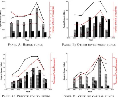
commodity trading advisors(“CTAs”) and commodity trading operators (“CTOs”). Figure 1.3 is split into four panels. Panels A, B, C and D display hedge funds, other investment funds, private equity funds, and venture capital funds, respectively. Focusing on the difference between the fundraising channels, the figure visualizes the amount of capital that was raised by directly-sold and broker-sold funds over the considered period.

To estimate the amount of capital inflows, I use reported information on the

Total Amount Sold that the fund reports in form D filings. I consider two cases:

capital inflows at the fund’s inception and capital inflows during the life of the fund. In the first case, the amount of capital raised at inception is directly reported in the Total Amount Sold variable. In the second case, it may be estimated as an increment of the Total Amount Sold variable between two consecutive fund’s filings. I outline the methodology on capital inflows estimation in Appendix.

The hedge fund industry enjoyed capital inflows which steadily grew from 2010 to 2015, spiking above the average level in 2014 and recovering to the previous trend of inflows at $300 billions per year. The spike in capital inflows in 2014 coincides with the lifting of the SEC’s advertisement ban, which was implemented in September 2013, following the JOBS Act directive.

1.1.2

Morningstar database and risk-adjusted returns

I use the Morningstar CISDM hedge fund database available from Wharton Re-search Data Service (“WRDS”). The database contains fund-level information on live and liquidated hedge funds. It keeps the most recent snapshot of fund’s adminis-trative information, such as name, address, inception date, compensation structure, minimum investment size, and liquidity restrictions. It also records the fundâĂŹs after-fee performance and assets under management at a monthly frequency.

monthly excess return,Re

it, on seven tradable risk factors, as suggested by Fung and

Hsieh (2004):

R_ite =αi+βM kt·SNP MRFt+βSmB ·SMBt+βT10y ·BD10RETt+

βCr.Spr.·BAAMT SYt+βpBD·P T F SBDt+βpF X·P T F SF Xt+

βpCOM·P T F SCOMt+ ˜ǫit.

(1.1)

To account for market exposure, I use annualized returns on the S&P500 index,

SNP MRFt. Adjusting for exposure to the size factor, I use an annualized return

spread between the Russell 2000 and the S&P500 index, SMBt, obtaining a time

series for the Russell 2000 and the S&P500 indexes from Thomson Reuters Datas-tream.

To control for yield curve exposure, I follow the literature and use the annualized excess returns of the U.S. 10-year Treasury constant maturity bond,BD10RETt. A

tradable yield curve level factor that is used in this paper is Bank of America Merrill Lynch’s U.S. 10-year Treasury constant maturity bond returns, which I download from Thomson Reuters Datastream. As a robustness check I used 10-year discount factors from the Federal Reserve Bank of St.Louis’ Treasury yield curve estimates.4

The correlation between the two time series is 0.96.

Accounting for credit spread exposure, I use an annualized return spread between Moody’s Baa-rated corporate bond, BAAMT SYt, and the U.S. 10-year Treasury

constant maturity bond. To proxy Moody’s Baa-rated corporate bond, I use the tradable Barclays Long Baa U.S. Corporate index, which can be downloaded from Thomson Reuters Datastream.

Finally, adjusting for the dynamic nature of the hedge funds’ strategies, I fol-low Fung and Hsieh (2004) and use a trend-folfol-lowing bond factor, P T F SBDt, a

trend-following currency factor, P T F SF Xt, and a trend-following commodity

fac-4_{FED’s yield curve can be downloaded from Federal Reserve Economic Data (FRED):}

tor, P T F SCOMt, which are constructed from look-back options and can be

down-loaded from David A. Hsieh’s Data Library.5

For every fund iin month t, I estimate its annualized monthly alpha, ˆαit, with a

two-year rolling-window regression (1.1). The final sample consists of 29,051 fund-month observations.

Although, investors care about after-fee returns on their hedge fund investment, skills of funds are reflected in pre-fee returns. Hedge fund databases usually take the perspective of investors and report fund performance and net asset values (“NAV”) after accounting for fees. To reconstruct pre-fee returns, I apply the modification of methodology that was used in Brooks, Clare and Motson (2007), Hodder, Jackwerth and Kolokolova (2012), and Kolokolova (2010)

I make several assumptions that reflect the general practice on the calculation of hedge funds’ fees. [1] Pro-rata management fees are paid at the end of the month on pre-fee net asset value at the end of the month. [2] Incentive fees are accrued on a monthly basis, but are only paid at the end of the calendar year; reported after-fee net asset value and performance account for accrued incentive fees. [3] Hedge funds use the high-watermark provision and incentive fees are paid in case pre-fee net asset value adjusted for management fees are above the current high water mark. [4] The high-water mark is reset to a pre-fee net asset value if it exceeds the current high water mark; otherwise the high-water-mark stays as in the previous month. [5] Management and incentive fees remain constant over time.6 _{[6] The equalisation}

credit/contingent redemption scheme is used to calculate net asset value to ensure that the fund managers are compensated correctly for positive performance, while investors, who might invest in funds at different time are treated fairly and equally.7

For each fund I estimate the pre-fee net asset value, NAV∗_{(t), and the} pre-fee return, R∗_{(t), using available data on after-fee net asset value, NAV(t),} after-fee return, R(t), management fee (in percentage terms), fM, and incentive fee (in

5_{David A. Hsieh’s Data Library is accessible at https://faculty.fuqua.duke.edu/ dah7/HFRFData.htm.} 6_{In reality hedge funds may update their compensation structure as documented by Deuskar}

et al. (2011), Agarwal and Ray (2012) and Schwarz (2007).

7_{âĂŸEqualisation Credit/Contingent RedemptionâĂŹ accounting procedure is described and}

The hedge fund database reports after-fee net asset value, which is calculated as a pre-fee net asset value adjusted for management fees (in dollars), FM(t), and

accrued incentive fees (in dollars), FI(t):

NAV(t) =NAV∗_(t)

−FM(t)−FI(t). (1.2)

Dollar management fees are calculated based on the net assets of the fund at the end of the month, as per assumption [1]:

FM(t) =NAV∗(t)·fM/12. (1.3)

Incentive fees accrue if the net asset value after management fees and net capital flows are above the high water mark, following assumptions [2], [3], and [4]:

FI(t) = max(0;NAV∗(t)−FM(t)−Netflows(t)−HWM(t))·fI. (1.4)

Solving the system of equations (1.2), (1.3), and (1.4), I express the pre-fee net asset value, dollar management fees, and the dollar incentive fees

                        

NAV∗_{(t) =}

NAV(t) +FM(t) +FI(t) (1.5)

FM(t) = [NAV(t) +FI(t)]·

fM/12

1₋fM/12

(1.6)

FI(t) = [NAV(t)−Netflows(t)−HWM(t)]·

fI

1₋fI·

I[NAV(t)₋Netflows(t)_>HWM(t)]

(1.7)

Dollar incentive fees (1.7) are accumulated only if the assets of the fund are above the high water mark, NAV(t)₋Netflows(t) > HWM(t); otherwise, the fund does not get any incentive fees.

under management at the end of the month, adjusted for dollar netflows during the period:

1 +R∗_{(t) =} NAV ∗_(t)

−Netflows(t)

NAV∗(t₋1)_−F

M(t−1)

. (1.8)

At the beginning of the investment period, assets under management are equal to pre-fee net assets at the end of the previous period adjusted for management fees. Also, the pre-fee net asset value has to be adjusted for netflows, which I estimate as in the literature on fund flows ( Sirri and Tufano (1998), Agarwal, Daniel and Naik (2004)).

Netflows(t) =NAV(t)₋NAV(t₋1)_·(1 +R(t)). (1.9) Finally, Substituting (1.2) and (1.9) into (1.8), I estimate the pre-fee return R∗(t).

1.1.3

Matching form D filings and Morningstar database

I match the form D filings with Morningstar database by the name of the fund using a fuzzy matching method.

First, I estimate the pairwise generalization of Levenshtein (1966) edit distance, a measure of dissimilarity, between the funds in Form D and Morningstar databases. I eliminate the pairs that have a dissimilarity score above 200. Second, I eliminate pairs of matched form D and Morningstar funds that report inception dates of more than six months apart from each other. Finally, I manually verify the results of the matching procedure.

14,581 form D filings, using the Hedge Fund Research (HFR) and Lipper TASS databases. The match rate between the form D funds and Morningstar funds is consistent with the match rates of form D funds with hedge funds that report to TASS (1,896 funds).

In the matched sample there are 1,103 of directly-sold funds and 625 of broker-sold funds.

Focusing on the heterogeneity of brokers, I further differentiate the broker-sold funds into funds that are offered to investors through in-house brokers and funds that are sold to by outside brokers. In the matched sample of broker-sold funds I identify in total 537 funds that are sold by outside brokers, 56 fund that are sold by in-house brokers and 32 funds that are sold through both.

The matched database inherits all the biases that are usually associated with Morningstar database.

First, the information that hedge funds report to Morningstar database is not verifiable. Fund managers usually list their funds in hedge fund databases to market their funds and attract potential investors. Agarwal, Mullally and Naik (2015) and Getmansky, Lee and Lo (2015) provide a comprehensive review of the limitations and potential biases in hedge fund data.

Often funds backfill returns prior to the date when they starts reporting to the data vendor. Thus, a fund manager has an incentive to list his hedge fund in a database after a period of good performance. As discussed in Edwards and Park (1996), this potentially leads to misleadingly good track records and may result in upward bias in expected returns due to this instant history or backfill bias.

Joenv¨a¨ar¨a, Kosowski and Tolonen (2014) estimate a backfill bias of around twenty months by analyzing snapshots of databases that have been taken on differ-ent dates. Following the literature practice, I exclude the first twdiffer-enty-four months of returns observations since the inception of the funds to mitigate this bias.

their performance after a period of bad performance. Therefore, underperforming funds may be under-represented, again biasing upwards the estimates of expected returns. To mitigate this bias, I consider both live and defunct funds moved to hedge fund graveyard files.

Third, Morningstar hedge fund data, unfortunately, contains significant numbers of missing assets under management. Following Joenv¨a¨ar¨a, Kosowski and Tolonen (2014), I fill in any missing observations with the most recent observations of the past.

Table 1.4 presents summary statistics on annual capital inflows, the number of investors, and the number of new investors across funds that are directly sold to investors and funds that are offered to investors through brokers from form D filings. Panel A presents the summary statistics for the whole sample of form D funds. Panel B presents summary statistics for the matched sample in order to examine any potential biases introduced by the matching procedure.

Annual capital inflows into hedge funds do not differ significantly across distri-bution channels. On average, directly-sold funds and broker-sold funds raise $49 millions per year. The median amount of capital raised by directly-sold funds is $3 millions and $5 millions for broker-sold funds. There are on average 12 investors in directly-sold funds and 33 investors in broker-sold funds. The average size of investment in a broker-sold fund is 2.75 less than that of a directly-sold fund.

I do not find significant differences between the matched sample and the total form D sample of funds, comparing a sample that consists of matched funds and sample of all form D funds on their observable characteristics.

1.2

Empirical evidence

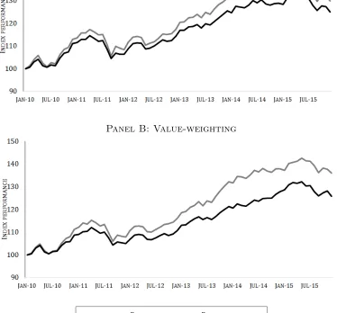
To compare the performance of funds between fundraising channels, I construct two portfolios of funds. The first one consists of directly-sold funds, representing the anti-intermediation view. The second one comprises hedge funds that are offered to investors through brokers, representing the pro-intermediation view. The port-folios of funds are rebalanced monthly, so that newly originated funds are included and liquidated funds are excluded appropriately. Assuming an initial investment of $100, I track the portfolios of the funds’ after-fee performance from January 2010 to December 2015.

Figure 1.4 plots the after-fee performance dynamics for the portfolios of funds. Panel A shows the performance of the portfolio of funds where the constituent funds are equally-weighted. Panel B displays the performance of portfolios of funds where the constituent funds are value-weighted. Portfolio of directly sold funds outperforms portfolio of broker sold funds over considered five year period. For the equally-weighted scheme, the portfolio of directly-sold funds increases from $100 to $130, with an annualized return of 5.38% per year over five years, while the portfolio of broker-sold funds rises from $100 to $125, with an annualized return of 4.56% per year. The difference is more pronounced when the value-weighted scheme is considered. Portfolio of directly sold funds increases from $100 to $136 with annualized return of 6.34% per year, while portfolio of broker sold funds increases from $100 to $126 with annualized return of 4.73% per year. The results also hold when I consider the full sample of hedge fund returns without adjusting for backfill bias. I present the results in Figure 1.7 in the Appendix.

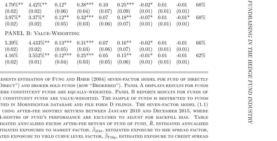
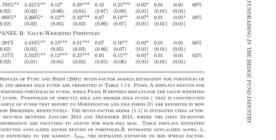
after-fee alpha of directly-sold hedge funds is persistently higher than the after-fee alpha of the broker-sold hedge funds regardless of portfolio-weighting scheme. For the equally-weighted scheme, the after-fee alpha of the directly-sold hedge funds is equal on average to 4.42% per year versus 3.37% per year for the broker-sold hedge funds. For the value-weighted scheme, the average alpha of the portfolio of directly-sold funds is equal to 4.43% as opposed to 3.55% for the portfolio of broker-directly-sold funds.

I implement another robustness check and perform panel data analysis. For each hedge fund i in month t, I estimate its annualized monthly alpha, ˆαit, with a two

year rolling-window regression (1.1). Then I estimate the difference between the alphas of the directly-sold funds and the broker-sold funds with a panel regression

ˆ

αit=β0+βB·Bit+βX ·Xit−1+βt+ ˜ǫit, (1.10)

where Bit is a dummy variable that is equal to one if fund i is sold through brokers

and it is equal to zero if the fund raises capital directly. I use a set of controls,Xit−1,

which includes the assets under management of hedge fund in a previous month, the age of the fund, and its vintage. I also control for aggregate demand shocks with time fixed effects, βt. The coefficient of interest that measures the difference in the

alphas of directly-sold and broker sold-funds is βB.

Panel A of Table 1.7 presents the results of the estimation of regression (1.10). I find that the after-fee alpha of the broker-sold funds is, on average, 1.6% per year lower than that of directly-sold funds. The results are economically significant and robust for inclusion of the fund’s size, age, vintage year controls and time fixed effects. I also find consistent results (reported in Appendix Table 1.16) for the sample of funds without correction for backfill bias.

I also compare the dollar value added measure of Berk and van Binsbergen (2013) for directly-sold funds and that of broker-sold funds. I find monthly dollar value added to investors, ˆSit, as a product of the after-fee alpha of the hedge fund and

receive, on average, $210,000 per month less than investors in directly-sold funds. The results are robust when controlling for the age of the fund, its vintage and time fixed effects.

Exploiting heterogeneity across brokers, I analyze the difference in performance between funds that are sold by in-house brokers and funds that are offered by outside brokers. I perform a formal analysis with the following panel regression:

Yit =β0+βI·BitI +βO·BOit +βX ·Xit+βt+ ˜ǫit, (1.11)

where Yit = ˆαit denotes the fund’s annualized risk-adjusted performance. BitI is a

dummy variable that is equal to one when the fund is offered to investors by an in-house broker and is equal to zero otherwise. BO

it is a dummy variable that is

equal to one when the fund is sold to investors through an outside broker and is equal to zero otherwise.

Table 1.9 displays the results of the estimation of regression (1.11). I find that the result of the under-performance of broker-sold funds is mostly driven by funds that are sold through in-house brokers. The average after-fee alpha of funds that are sold through in-house brokers is 2% lower than that of directly-sold funds, while average after-fee alphas of funds that are offered through outside brokers is 1.4% lower than that of directly sold funds. Performing a formal F-test and comparing the difference between in-house broker-sold and outside broker-sold funds, I find that the alpha of funds that are sold by in-house brokers is statistically different from the alpha of funds that are sold by outside brokers. The results are robust when the fund’s size, vintage, and year-month controls. Furthermore, I perform additional robustness checks by estimating the regression (1.11) on the sample that does not correct for backfill bias, which is displayed in Table 1.18 in the Appendix.

broker-sold mutual funds, with an average after-fee alpha of -2.28% per year, underperform directly-sold mutual funds, with an average after-fee alpha of -1.07% per year, by 1.21% per year. Del Guercio and Reuter (2014) and Reuter (2015) find similar results when considering different weighting schemes. Authors document the difference in equally-weighted after-fee alphas between the two groups of funds of 1.15% and that of the value-weighted after-fee alphas 0.64% per year. Christoffersen, Evans and Musto (2013) find that a 1% increase in the excess load paid to broker decreases mutual fund after-fee future performance by 0.24% over the next year. In contrast to my results, the authors find that the underperformance is mostly driven by mutual funds that are sold through outside brokers rather than in-house brokers.8

1.2.2

Pre-fee performance across distribution channels

Addressing the question of whether brokers help to identify skillfull hedge funds, I analyze the pre-fee risk-adjusted performance of funds across distribution channels. I estimate the two-year rolling pre-fee alpha of portfolios of funds, adjusting their pre-fee returns for systemic risk exposure using equation (1.1). Figures 1.6 presents the time-series dynamics of the pre-fee alphas of the portfolio of directly-sold funds and the portfolio of broker-sold funds. The figure is split into two sub-figures, which correspond to the equally-weighted scheme in Panel A and the value-weighted scheme in Panel B.

The pre-fee alpha of the portfolio of directly-sold hedge funds is persistently higher than the pre-fee alpha of the portfolio of broker-sold hedge funds regardless of the portfolio-weighting scheme. I find that for the equally-weighted scheme, the alpha of the portfolio of directly-sold hedge funds is equal, on average, to 5.78% versus 4.48% per year for the portfolio of broker-sold funds. For the value-weighted scheme, the average alpha of directly-sold funds is equal to 5.53% versus 4.95% for the broker-sold funds.

I implement another robustness check and compare the skill of the funds across

8_{Christoffersen, Evans and Musto (2013) refer to outside brokers as non-affiliated brokers and}

the estimation results of the panel regression. I find that the funds that are sold to investors through brokers underperform funds that are offered to investors directly by 2% per year before accounting for fees. The results are robust for the inclusion of fund-level controls and time fixed effects. I perform a robustness check, using sample without adjusting for backfill bias and find consistent results reported in Panel B of Table 1.16 in the Appendix.

I also compare the dollar value added by directly-sold hedge funds and broker-sold hedge funds. I find the monthly dollar value added of the hedge fund as a product of the pre-fee alpha of the hedge fund and its assets under management in a given month. The dollar value added measure estimates the amount of money that the hedge fund extracts from the financial markets. I perform a panel data analysis and report the results in Panel B of Table 1.8. I estimate that the value added by a broker-sold fund is, on average, $190,000 per month lower than the value added by a directly-sold hedge fund. The result is robust in controlling for the age of the fund, its vintage and the time fixed effects.

1.2.3

Fees across distribution channels

Next, I assess whether intermediaries help investors to find funds that charge lower fees. To answer this question, I use information about management fees and in-centive fees that hedge funds report in Morningstar database. Since only the most recent contract characteristics are kept in the database, I perform a formal compar-ison using the following cross-sectional regression:

Yi =β0+βB·Bi+λt+ ˜ǫi, (1.12)

where Bi is a dummy variable that is equal to one when fund is broker-sold and

is equal to zero otherwise. The regression includes a control for the fund’s vintage year, λt.

Table 1.11 compares the fees of hedge funds across the distribution channels. Columns (1) and (2) estimates the difference in the management fees of broker-sold and directly-sold hedge funds. On average, hedge funds charge their investors 1.4% management fees, but I do not find any significant difference between funds with different distribution channels. I also do not find any significant difference between the management fees that funds sold through in-house brokers and funds offered through outside brokers charge their investors. These results are not surprising since hedge funds uses management fees to cover their operational expenses.

Chalmers and Tufano (2009) establish that the non-distributional expenses of mu-tual funds that are sold through intermediaries are 23 basis points higher than those of mutual funds that are sold to investors directly, concluding that brokers do not help investors to identify mutual funds with lower non-distribution fees.

1.2.4

Clientele across distribution channels

I complete the empirical analysis by analyzing whether investors of broker-sold hedge funds differ from investors of directly-sold hedge funds. Since hedge funds are very secretive and do not disclose information about their investors, I use a minimum investment size and an average investment size as empirical proxies of the size of the hedge fund’s marginal investor and average investor. To estimate the difference in the hedge funds’ clientele across the distribution channels, I estimate a regression (1.12).

Columns (1) and (2) of Table 1.12 estimate the difference in the minimum invest-ment size of broker-sold and directly-sold hedge funds. The minimum investinvest-ment size of directly-sold funds is, on average, $1 million, which is $0.27 millions more than that of directly-sold funds. Further, analyzing the heterogeneity of brokers, I find that the minimum investment size of funds sold through in-house brokers does not differ from that of directly-sold funds, while the minimum investment size of funds sold through outside brokers is $0.21 millions lower than that of directly-sold funds. Performing an F-test, I find that the minimum investment size of in-house broker-sold funds is statistically different from the minimum investment size of out-side broker-sold funds.

Columns (3) and (4) of Table 1.12 estimate the difference in the average in-vestment size of broker-sold and directly-sold hedge funds. Comparing the average investment size, I find that broker-sold funds have a $12 millions lower average investment size than directly-sold funds.

1.3

Theoretical motivation

I presents a simple model of fundraising in the hedge fund industry. I then reconcile empirical findings with the model implications and estimate the compensation that brokers receive for capital introduction services.

1.3.1

Model of fundraising

Suppose there are three types of agents: hedge funds, investors, and brokers, who intermediate between hedge funds and investors. There are two risk-neutral funds that differ in their portfolio management skills: a good fund and a bad fund. Let

θ denote a type of fund, where θ _{∈ {}G, B_} corresponds to the good fund and the bad fund, respectively. The good and the bad funds deliver positive pre-fee risk-adjusted returns,αG andαB, respectively, with αG > αB>0. I assume that alphas

are known to the funds themselves, but unobservable to investors and the broker. The fund does not have capital and has to raise it from investors. It can either directly raise capital from investors or use capital introduction services offered by the broker. For its portfolio management services, the fund charges performance-based fees, which are calculated as the fraction of generated profits. The fund chooses a fee and capital raising channel to maximize the total dollar fees that it collects from its investors.

There is also a continuum of risk-neutral investors. Each investor is endowed with a unit of capital, which he may either invested in one of the hedge funds or in an outside option (return of the outside option is normalized to zero). All investors qualify for the status of accredited investor and may invest in hedge funds. To capture heterogeneity among clientele, I assume that investors differ in their search and due diligence costs. There are professional investors with low search and due diligence costs and mainstream accredited investors who have high search and due diligence costs. I assume that the search and due diligence costs of investors, c, are uniformly distributed at interval from 0 to ¯C, c_∼U[0; ¯C].

broker and invest his money into a fund recommended by the broker. In the latter case, the broker performs due diligence and certifies the quality of the fund.

Due diligence is important since the hedge fund industry is opaque and there are fraudulent funds that investors should be aware of. Analyzing form ADV disclosures of registered hedge funds, Brown et al. (2008) find that approximately 16% of hedge funds have committed a felony or have financial-related charges or convictions. As pointed out by Garleanu and Pedersen (2016), hedge fund prospective investors usually undertake extensive analysis by studying the track record and evaluating the investment process and the risk management of funds. Fraudulent, negative alpha funds exist on the off-equilibrium path. Therefore, investors who do not perform due-diligence may loose money investing in these funds.

The broker performs due diligence and a certification of the fund at cost, cI >0.

For the capital introduction service, the broker charges the fund some fraction of the fund’s fees. The broker and the fund bargain with each other and split the collected dollar fees. I assume that the bargaining power of the broker is an exogenous parameter, G _∈ (0; 1). Although I do not solve for an optimal contract for the broker, the performance-related compensation ensures that the broker acts in the interest of investors and allows for avoiding a moral hazard problem between the broker and the investors.

The fundraising game has a simple sequential structure, which is illustrated in Figure 1.1. At time 1, the good fund and the bad fund simultaneously announce fees that they charge for portfolio management services and their choices of capital raising channels. At time 2, the investors decide whether to invest into the hedge fund industry on their own or hire an intermediary broker.

Strategies.

Letfθbe a fee that a type-θfund charges its investors. LetXθbe the fund’s choice of

capital raising channel. If the type-θ fund is sold to investors directly then Xθ = 0.

If the type-θ fund is sold to investors by the broker, then Xθ = 1. The strategy of

Figure 1.1: Time line of the fundraising game

bad fund have strategies sG and sB, respectively.

The investor decides either to perform a costly due diligence of the hedge fund industry at cost c and invest into one of the funds on his own or to approach the intermediary broker and follow his investment advice. In both cases, the investor pays a portfolio management fee, fθ, upon investing into the type-θ hedge fund.

The decision of the investor depends on his search and due diligence costscand the strategies of the funds sG and sB.

Payoffs of players.

Let’s denote the profit of type-θ hedge fund Πθ

sθ;s−θ;C(sθ, s−θ)

. It depends on the strategy of the type-θ fund sθ, the strategies of the other fund s−θ, and a

pro-portion of investors, who decide to invest in the fund, denoted asC(s_{θ, s−θ})_⊂[0; ¯C]. Given strategy sθ = (fθ, Xθ), the profit of the type-θ fund is determined as

Πθ

sθ;s−θ;C(sθ, s−θ)

= Πθ

(fθ, Xθ);s−θ;C(sθ, s−θ)

= (1.13)

    

   

fθ·

Z

C_(sθ,s

−θ)

dc, if Xθ = 0 (1.13a)

(1₋G)_·fθ·

Z

C(sθ,s−θ)

dc, if Xθ = 1. (1.13b)

If the type-θ fund decides to be sold to investors directly (Xθ = 0), then its profits

are equal to the total dollar fees raised from the investors, as in (1.13a). If the type-θ fund decides to be sold to investors through the broker (Xθ = 1), then the fund and

Let’s denoteUθcthe utility of the investor with due diligence costc, who allocates

his endowment into the type-θ fund. It is equal to

Uθc=αθ−fθ−c·I{Xθ = 0}. (1.14)

If the investor invests on his own, then his utility equals to the after-fee return of the type-θ fund adjusted for due-diligence costs. If the investor follows financial advice, then his utility equals to the after-fee return on the type-θ fund.

Let’s denote the profit that the broker gets ΠI

sθ;s−θ;C(sθ, s−θ)

. It is equal to the compensation that the broker gets for the capital introduction service adjusted for due diligence cost cI. The profit of the broker may be expressed in terms of the

profit that the fund receives as follows:

ΠI

sθ;s−θ;C(sθ, s−θ)

= G

1₋G·Πθ

sθ;s−θ;C(sθ, s−θ)

−cI

·I_{Xθ= 1_}. (1.15)

The broker makes a profit when the fund is broker-sold (Xθ = 1) and he gets no

profit when the fund is directly-sold to investors (Xθ = 0).

Definition of “cut-off” equilibrium.

I define the Nash equilibrium of the fundraising game as follows: (i) The good fund chooses strategy sG to maximize its profits

ΠG

sG;sB;C(sG, sB)

≥ΠG

s′

G;sB;C(s′G, sB)

for any

s′

G ∈R+× {0,1}/{s′G6=sG}.

(ii) The bad fund chooses strategy sB to maximize its profits

ΠB

sB;sG;C(sB, sG)

≥ΠB

s′

B;sG;C(s′B, sG)

for any

s′

B∈R+× {0,1}/{s′B6=sB}.

(iii) There is a cut-off marginal investor with due diligence cost ˆc(sθ, s−θ) who is

marginal investor, i.e. C(s_{G, sB}) =h0; min_{c(sˆ _{G, sB}),_C¯_}i will invest on their own. Investors with costs that are greater than the cost of the marginal investor, i.e

C(s_{B, sG}) =min_{ˆc(s_{B, sG}),_C¯_}; ¯_Ci will approach the broker for investment advice. (iv) The profit of the broker covers his due diligence cost, ci.

Note that I restrict a space of the investor’s strategies to “cut-off” strategy, which is determined by the marginal investor with a search and due diligence cost, ˆc(sθ, s−θ).

Since the investors base of the fund C(s_{θ, s−θ}) may be fully described by a thresh-old search and due-diligence cost ˆc(sθ, s−θ) of the marginal investor, it allows me

to simplify the notation for the profit of the type-θ fund in the following way, Πθ

sθ;s−θ; ˆc(sθ, s−θ)

.

PROPOSITION. There exists a separating pure strategies “cut-off” equilibrium in

the fundraising game. A good fund is directly-sold to investors and charges fee f∗

G =

αG

2 . A bad fund raises capital through a broker and charges fees f

∗

B =αB.

s∗

G=

α_G

2 ,0

, (1.16)

s∗

B =

αB,1

. (1.17)

A marginal investor with due diligence cost ˆc∗ _{gets zero utility and is indifferent}

between investing into the hedge fund industry on his own or using the investment

advice of a broker:

ˆ

c∗ ₌ αG

2 , (1.18)

UGc∗ =U_Bc∗ = 0. (1.19)

Investors with costs c < cˆ∗ _{invest by themselves and those with c > ˆc}∗ _{follow the}

The necessary conditions for the existence of separating equilibrium are as follows:

max1₋ αG

4_·C¯;

cI

αB·( ¯C−α₂G)

6G < 1 (1.20)

αB <ˆc∗ =

αG

2 <C.¯ (1.21)

This separating “cut-off” equilibrium of the fundraising game is illustrated in Figure 1.2.

Figure 1.2: Separating equilibria of the fundraising game

Solution.

I verify the existence of the separating “cut-off” equilibrium by confirming the op-timality of strategies of the players’ strategies.

Good fund.

The good fund chooses optimally its fee and capital raising channel to maximize its profits (1.13). Since the capital raising choice of the fund is binary, the profit maximization over a two-dimensional vector-strategy sG = (fG, XG) simplifies to

to the choice by the good fund of engaging in direct capital raising. The second optimization corresponds to a choice by the good fund of raising capital through the broker.

First, let’s calculate the profits that the good fund gets if it chooses to be directly-sold (Xθ = 0). Its investor base includes either all the investors with due

dili-gence costs that are smaller than threshold ˆc or the entire population of investors,

C(s_{G, sB}) = h0;_min{c(sˆ _{G, sB}),_C¯_}i. The good fund chooses fee _fG to maximize its profits subject to the feasibility condition on fees and the participation constraint of the marginal investor.

ΠG

(fG,0);sB; ˆc(sG, sB)

= max

fG

fG·

Z min n

ˆ

c((fG,0);sB),C¯

o

0 dc

(1.22)

subject to

06fG 6αG (1.22a)

αG−fG−ˆc((fG,0);sB) = 0. (1.22b)

The fee feasibility constraint (1.22a) states that the fund can not charge a fee fG

that is bigger than the return αG that it generates. The participation constraint

(1.22b) says that the marginal investor has to be indifferent about receiving utility

αG−fG−cˆupon investment into the fund and the utility of zero upon investment

in an outside option.

max

fG

fG·(αG−fG) (1.23)

subject to

06fG 6αG. (1.23a)

The hedge fund’s choice of fee affects its profits directly through feefGand indirectly

through the size of its investors baseαG−fG. The good fund exercises its monopoly

power and sets a fee optimally at, fG = α₂G. Thus, the strategy of the good fund

that chooses to be sold to investors directly is sG = (α₂G,0) and its profits are:

ΠG

(αG

2 ,0);sB; ˆc(sG, sB)

= α2G

4 . (1.24)

The threshold search and due diligence costs are equal to

ˆ c= αG

2 . (1.25)

To ensure the interior case occurs, which makes it suboptimal for high-cost investors to invest on their own, the following condition has to be satisfied:

ˆ

c <C.¯ (1.26)

Substituting (1.25) into (1.26), I get the second condition in (1.21).

Second, let’s calculate the profits that the good fund gets if it chooses to be sold through broker (XG = 1). In this case, both funds are offered to investors through

a broker. However, the broker will only market the good fund, since in this case, he will receive higher compensation. Thus, all investors will be channelled to the good fund and C(s_{G, sB}) = [0; ¯C]. The good fund that is sold through the broker will choose fee fG to maximize its profits subject to the feasibility condition on the fee

ΠG

(fG,1);sB; ˆc(sG, sB)

= max

fG

(1₋G)_·fG·

Z C¯

0 dc

(1.27)

subject to

06fG 6αG (1.27a)

G_·fG·

Z C¯

0 dc

>cI. (1.27b)

The fee feasibility constraint (1.27a) is similar to (1.22a). The broker helps to attract all investors to the good fund and gets a fraction G of the total dollar fees. The participation constraint of the broker (1.27b) ensures that the compensation that he receives is enough to cover his due diligence cost cI.

Since the good fund gets all the investors regardless of the fees that it charges, it optimally sets a fee to extract all profits, leaving investors indifferent about investing into the fund or investing into the outside option. Thus, the good fund that chooses to be sold to investors through the broker sets fee fG =αG. Its optimal strategy is

sG = (αG,1) and its profits are equal to the (1−G) fraction of the generated surplus

αG·C.¯

ΠG

(αG,1);sB; ˆc(sG, sB)

= (1₋G)_·αG·C.¯ (1.28)

The profits of the broker equals the fraction G of the generated surplus after ac-counting for the due diligence costs of the broker.

ΠI

(αG,1);sB; ˆc(sG, sB)

=G_·αG·C¯−cI. (1.29)

ΠG

(αG

2 ,0);sB; ˆc(sG, sB)

>ΠG

(αG,1);sB; ˆc(sG, sB)

. (1.30)

Substituting (1.24) and (1.28) into condition (1.30) gives the first constraint on the bargaining power (1.20) of the broker:

G_≥1₋ αG

4_·C¯. (1.31)

Bad fund.

The bad fund optimally chooses a fee and capital raising channel which maximizes its profits (1.13). Similar to the analysis for the good fund, I consider two separate cases, which correspond to the choice of fundraising of the bad fund.

First, let’s calculate the profits that the bad fund gets if it chooses to be sold to investors through broker (XB = 1). Investors with search and due diligence

costs c >cˆapproach the broker and invest their capital in the fund that the broker recommends. Its investor base is C(s_{B, sG}) = (ˆc(s_{B, sG}); ¯C] for the interior case when ˆc < C. The bad fund chooses fee¯ fB to maximize its profit subject to the

feasibility condition on the fee and the participation constraint of the broker.

ΠB

(fB,1);sG; ˆc(sB, sG)

= max

fB

(1₋G)_·fB·

Z C¯

ˆ

c(sB,sG)

dc (1.32)

subject to

06fB 6αB (1.32a)

G_·fB·

Z C¯

ˆ

c(sB,sG)

dc>cI. (1.32b)

The fee feasibility constraint (1.32a) states that the fund cannot charge a fee fB

bigger than the returnαBthat it generates. The broker brings investorsC(sB, sG) =

(ˆc(sB, sG); ¯C] to the bad fund and receives a fractionG of the total dollar fees that

the compensation that he receives is enough to cover his due diligence cost cI.

The choice of fees of the bad fund has only a direct effect on its profit, since its investors’ base comes from the broker. Thus, it maximizes its profits by extracting all profits through fees and making its investors indifferent about investing into the fund or investing in an outside option. Thus, the bad fund that chooses to be sold to investors through the broker sets the fee fB = αB. Its strategy is sB = (αB,1)

and its profits are equal to the (1₋G) fraction of the generated surplusαB·[ ¯C−α₂]

ΠB

sG; (αB,1); ˆc(sB, sG)

= (1₋G)_·αB·[ ¯C−

αG

2 ]. (1.33)

The profits that the broker gets is a fraction G of the generated surplus after ac-counting for the due diligence costs of the broker.

ΠI

sG; (αB,1); ˆc(sB, sG)

=G_·αB·[ ¯C−

αG

2 ]−cI >0. (1.34)

Condition (1.34) yields the second constraint (1.20) on the bargaining power of the broker.