2016 International Conference on Electronic Information Technology and Intellectualization (ICEITI 2016) ISBN: 978-1-60595-364-9
Analog Circuit Diagnosis Based on
SubKPCA-SVM
Bin Peng and Zhemin Duan
ABSTRACT
In analog circuit diagnosis, too many variables increase computing times and result in real-time performance degradation. In this paper, SubKPCA have been proposed to extract the effective feature, on this basis, SVM is introduced to establish the diagnosis model. Analog circuit fault diagnosis experiments on CTSV filter verify the effectiveness and accuracy of the proposed method.
INTRODUCTION
Fault diagnosis for analog circuit is still a challenging subject in the circuit test research field. Due to the inherent characteristics of analog circuit [1-2], such as its nonlinearity, continuous response and tolerance on component parameters, etc., inducing the diversity and complexity of fault types of the circuit, it is difficult for the conventional fault diagnosis theories and methods to achieve the expected results in practical engineering. Hence, it is very important to explore some efficient fault diagnosis theories and methods to meet the development of analog circuit.
In recent years, Support Vector Machines (SVM) has achieved a great development for its application in various fields [3-5]. In this paper, we use SVM to meet challenges in analog circuit diagnosis. The relevant, nonlinear and redundant features variables in actual fault diagnosis system for analog circuit spoil SVM's classification performance seriously. Too many variables increase computing time and result in real-time performance degradation. Feature extraction can solve these
_______________________
problems well. Principal Components Analysis (PCA) can extract the principal components [6], but it only deals with linear problems, as a nonlinear problem, PCA are not suitable in analog circuit diagnosis. To solve nonlinear problems, Kernel Principal Components Analysis (KPCA) was developed. But it needs to calculate the kernel matrix. The more the samples quantity, the larger the kernel matrix [7-8].This uses plenty of computation and time source. For this problem, Y. Washizawa proposed the Subset KPCA (SubKPCA) which applies the clustering method to choice a subset from the training sample set for kernel matrix. This method can improve the computation speed in evidence, and can achieve the same effect as KPCA as a whole [9-10].
On this basis, we propose a new fault diagnosis method: SubKPCA-SVM. The Subset KPCA feature extraction is organically integrated with SVM in order to improve the efficiency and accuracy of fault diagnosis for analog circuit. Simulation results validate the effectiveness.
SUBSET KPCA
The basic idea of SubKPCA is that, as KPCA is conducted, a subset of the training samples is selected in advance, by appropriate optimization in order to achieve a similar analysis effect using all the training samples. The steps of Subset KPCA feature extraction are as follows:
1. A sample subset Y is selected from the training samples X. 2. The matrix Ky and
T
xy xy
K K are calculated.
3. The generalized eigenvalue decomposition to ( 1/2) T ( 1/2)
y xy xy y
K K K K is
conducted to obtain r eigenvalues 1, , ,2 r from large to small and also to get the corresponding eigenvector VSKPCA [ , , , ]v v1 2 vr .
4. Store [( 1/2) ]T
y SKPCA
K V and all subset samples.
5. According to the following formula, the empirical kernel map hx of input
vector x is calculated.
hx[ ( , ), ( , ), , ( ,k x y1 k x y2 k x ym)] (1)
6. Use the following formula to transform hx.
( ) [( 1/2) ]T
SKPCA x y SKPCA xh
U K V (2)
7. The main calculation from Step 1 to Step 3 is the generalized eigenvalue decomposition. The size of the eigenvalue decomposition for KPCA is n, and the
computational complexity from Step 4 to Step 5 mainly depend on the size m of
the determined subset, and the memory required for saving [( 1/2) ]T
y SKPCA
K V and all subset samples is also reduced. It also means that, for input vector x, the
system response time of Subset KPCA is less than that of KPCA.
SVM CLASSIFIER
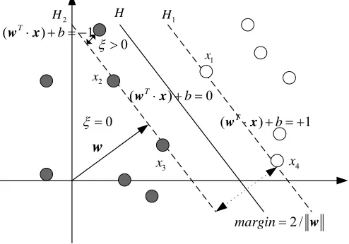
SVM classifier is a supervised learning algorithm based on statistical learning theory, whose aim is to determine a hyper plane that optimally separates two classes by using train data sets [11]. Consider a classification problem with the dataset
1 1 2 2
{( , ),( , ), ( , )}l l
D x y x y x y , where m i
x R andyi { 1, 1}. The optimal separating hyper plane:
: T 0
H w x b (3)
where bR is the bias term and wRm is the normal vector to the hyper
planes. The hyper plane described by (3) lies midway between the bounding hyper planes given by:
1: T 1
H w x b ; 2: 1
T
H w x b (4)
The optimum separating hyper plane can be found by minimizing
2 w
(or w wT ) under the constraint yi(wTxib) 1 i, i 0,i1, , l iR is the soft margin error of the ith training poin Thus, determination of optimum hyper-plane is required to solve optimization problem given by:
,
1
1 min
2
. . ( ) 1 , 0, 1, , l T i b i T
i i i i
C
s t y b i l
w w w
w x
(5)
Where C is a regularization constant or penalty parameter, which controls the tradeoff between the two competing criteria of margin maximization and error minimization. Thus, the classification decision function becomes:
: T 0
H w x b (6)
nonlinear mapping functions ( ) xi . The classification process of SVM is shown in Figure 1.
1
H
2
H H
2 /
margin w
w
1
x
2
x
3
x x4
0
0
(wTx) b 1
(wTx) b 0
( T ) 1
b
w x
Figure 1. The classification process of SVM.
EXPERIMENTAL ANALYSIS FOR ANALOG CIRCUIT DIAGNOSIS
The process of the analog circuit diagnosis based on SubKPCA-SVM is shown in Figure 2. Firstly, we extract the fault features from fault database. In the study, SubKPCA technology is applied to extract the feature of analog circuit fault. Then, based on these extracted features, the diagnosis model is established by SVM training. As the real time fault data is collected, this data is transferred to extracted features by SubKPCA, and then sent into the diagnosis model to get fault types.
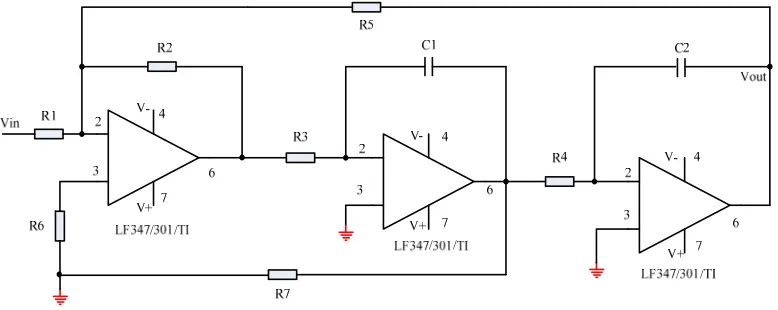
[image:4.612.96.494.555.630.2]In the study, we employ the international standard circuit: CTSV filter circuit [12] to study the fault diagnosis performance of SubKPCA-SVM compared with SVM, PCA-SVM and KPCA-SVM. The CTSV filter circuit is shown in Figure 3, in the circuit, as R1=R2=R3=R4=R5 =10kΩ,R6=3kΩ,R7=7kΩ,C1=C2=20nF.
Figure 3. CTSV filter circuit.
In the experiment, 8 fault types: F1(R1+50%), F2(R1-50%), F3(C1+50%), F4(C1-50%), F5(C2+50%) , F6(C2-50%) , F7(R5+50%), F8(R5-50%) are set. Here, the ‘+’ and ‘-’ represent the component value is set to upward or downward compared to the standard value, adding the normal state, there are 9 states. The pumping signal Vin is subjection, linear voltage, with the coordinate ((0,0); (0.5ms,5V); (1ms,-5V); (1.5ms,5V); (3ms,5V)). The CTSV filter is simulated by Orcad 10.5, and all 9 states are analyzed by Monte-Carlo method. In the experiment, while the pumping signal is imported, the Vout is measured and collected. Each simulation collects 400 samples at a certain intervals (for example 1us), and every state simulates 100 times. Training samples are randomly selected and residual are testing samples.
EXPERIMENTAL RESULT AND ANALYSIS
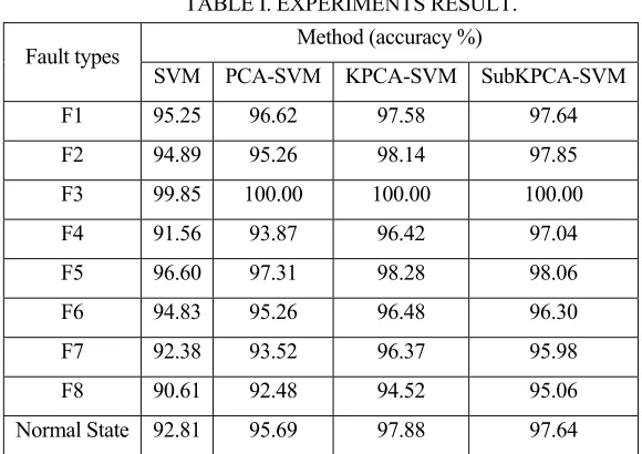
TABLE I. EXPERIMENTS RESULT.
Fault types Method (accuracy %)
SVM PCA-SVM KPCA-SVM SubKPCA-SVM
F1 95.25 96.62 97.58 97.64
F2 94.89 95.26 98.14 97.85
F3 99.85 100.00 100.00 100.00
F4 91.56 93.87 96.42 97.04
F5 96.60 97.31 98.28 98.06
F6 94.83 95.26 96.48 96.30
F7 92.38 93.52 96.37 95.98
F8 90.61 92.48 94.52 95.06
Normal State 92.81 95.69 97.88 97.64
As can be known from TABLE I, these four methods can diagnosis circuit fault well. SVM gets the lowest diagnosis accuracy, because there are relevant, nonlinear and redundant features variables. PCA-SVM’s accuracy is better than SVM, because through PCA processing, some relevant, redundant features are wiped off, the extracted features are more efficiency and accuracy. But the PCA can only deal with linear problems, as a no linear problem, PCA is not a suitably method. The KPCA-SVM and SubKPCA-KPCA-SVM get the best diagnosis accuracy, because they can solve the nonlinear problems well. From TABLEI, we can find the SubKPCA-SVM diagnosis accuracy almost equal to KPCA-SVM, but the extraction process is much easier than KPCA: both in computational process and memory requirement. These are very important in analog circuit diagnosis for its real-time requirement.
CONCLUSIONS
In this paper, we discuss a new method of analog circuit diagnosis: SubKPCA-SVM. The experiment result shows that, in the diagnosis accuracy, the proposed SubKPCA- SVM is equal to KPCA-SVM while it needs less computation and memory. As the real-time requirement in analog circuit diagnosis, SubKPCA-SVM is an effective method.
REFERENCES
1. Kabisatpathy P., Barua A., Sinha S. 2005. “Fault Aiagnosis of Analog Integrated Circuits,” Springer, Volume 30.
3. Jin Wei, Zhang Jian-qi, Zhang Xiang. 2011. “Face Recognition Method Based on Support Vector Machine and Particle Swarm Optimization,” Expert Systems with Applications, 38 (2011): 4390-4393.
4. Ji Zheng, Bao-Liang Lu. 2011. “A Support Vector Machine Classifier with Automatic Confidence and its Application to Gender Classification,” Neuro computing, 74 (11): 1926-1935. 5. A. Al-Anazi, I.D. Gates. 2010. “A Support Vector Machine Algorithm to Classify Lithofacies
and Model Permeability in Heterogeneous Reservoirs,” Engineering Geology, 114 (2010): 267-277.
6. Jolliffe I.T.. 2002. “Principal Component Analysis,” 2nd Ed. New York, USA: Springer.
7. Y. G. Fan, P. Li, Z.H. Song. 2005. “KPCA Based on Feature Samples for Fault Detection,” Control and Decision, 20 (12): 1415-1422.
8. B. Scholkopf, A. Smola, K.R. Muller. 1998. “Nonlinear Component Analysis As a Kernel Eigenvalue Problem,” Neural Computation,10 (5): 1299-1319.
9. Y. Washizawa. 2009. “Subset Kernel Principal Component Analysis,” Proceedings of 2009 IEEE International Workshop on Machine Learning for Signal Processing, Grenoble, France, September, (2009), 1-6.
10. Y. Washizawa. 2012. “Subset Basis Approximation of Kernel Principal Component Analysis,” Technical Report 2012-03, The University of Electro-Communications.
11. V. Vapnik. 1998. Statistical Learning Theory. New York: Wiley.