SIMULATIONS ON LÉVY SUBORDINATORS
AND LÉVY DRIVEN CONTAGION MODELS
Yan Qu
Department of Statistics
The London School of Economics and Political Science
A thesis submitted for the degree of
Doctor of Philosophy
Declaration
I certify that the thesis I have presented for examination for the PhD degree of the London School of Economics and Political Science is solely my own work other than where I have clearly indic-ated that it is the work of others (in which case the extent of any work carried out jointly by me and any other person is clearly identified in it). The copyright of this thesis rests with the author. Quotation from it is permitted, provided that full acknowledgement is made.This thesis may not be reproduced without my prior written consent. I warrant that this authorisation does not, to the best of my belief, infringe the rights of any third party.
Statement of conjoint work
I confirm that parts of Chapter3were adapted into a paper entitled "Exact Simulation of Gen-eralised Vervaat Perpetuities" jointly co-authored with Prof Angelos Dassios and Dr Jia Wei Lim, and is published inJournal of Applied Probability.
Acknowledgments
First and foremost, I would like to thank my supervisor Prof Angelos Dassios. My PhD journey would not have been such pleasant and enjoyable without his support, guidance, patience, and en-couragement over the years. His profound insights, enthusiasm and perseverance towards research have always given me momentum to progress. I really appreciate all his contributions of time for numerous discussions to make my work productive and stimulating, and for that I owe him many thanks.
I am grateful to my second supervisor Dr Erik Baurdoux for introducing me to the field of Lévy pro-cesses. His important suggestions and advice are invaluable. My thanks also goes to my examiners Prof Kostas Kardaras and Prof Andreas Kyprianou for giving me helpful comments to improve my thesis. I would like to extend my sincerest thanks to Dr Jia Wei Lim and Dr Hongbiao Zhao for many enlightening discussions and helpful suggestions during my PhD studies. I feel privileged and lucky to get the opportunity to work with them together.
I would like to thank the Department of Statistics at London School of Economics and Political Science for providing such a friendly working and teaching environment. Special thanks to my of-fice mates Andy Ho, Haziq Jamil, Pheonix Feng, Luting Li, Filippo Pellegrino, Alice Pignatelli Di Cerchiara, Ragvir Sabharwal, Tayfun Terzi, and Xiaolin Zhu for all the fruitful chats and enjoyable moments we have shared together.
Abstract
Contents
1 Introduction 9
I Exact Simulation on Lévy Subordinators 13
2 Lévy Subordinators 15
2.1 Definitions. . . 15
2.2 Compound Poisson Process . . . 17
2.3 Gamma Process . . . 17
2.4 Tempered Stable Process . . . 18
2.4.1 Tempered Stable Distributions . . . 20
2.4.2 Two-Dimensional Single Rejection Scheme . . . 21
2.4.3 Exact Simulation Scheme . . . 22
2.4.4 Numerical Experiments . . . 31
2.5 Conclusion . . . 33
3 Truncated Lévy Subordintors 35 3.1 Preliminaries . . . 35
3.2 Distributional Properties . . . 37
3.3 Marked Renewal Representation . . . 38
3.4 Dickman and Truncated Gamma Process . . . 40
3.4.1 Definitions and Distributional Properties . . . 40
3.4.2 Exact Simulation Scheme . . . 42
3.5 Truncated Stable Process . . . 45
3.5.1 Definitions and Distributional Properties . . . 45
3.5.3 Special Case: Truncated Inverse Gaussian Processes . . . 54
3.6 Numerical Experiments . . . 64
3.7 Applications in Finance and Insurance . . . 67
3.7.1 Exact Simulation of Generalised Vervaat Perpetuities . . . 67
3.7.2 Loss distributions with excess of loss reinsurance . . . 73
3.7.3 Pricing zero coupon Parisian bond . . . 78
3.8 Conclusion . . . 78
II Exact Simulation on Lévy Based Stochastic Models 81 4 Lévy Driven Ornstein-Uhlenbeck Processes 83 4.1 Introduction . . . 83
4.2 Distributional Properties . . . 84
4.3 Shot-noise process . . . 86
4.3.1 Laplace Transform . . . 87
4.3.2 Exact Simulation Scheme . . . 88
4.3.3 Simulation Studies . . . 89
4.4 OU-ΓProcess . . . 90
4.4.1 Laplace transform . . . 90
4.4.2 Exact Simulation Scheme . . . 91
4.4.3 Simulation Studies . . . 93
4.5 OU-TS Process . . . 94
4.5.1 Laplace Transform . . . 94
4.5.2 Exact Simulation Scheme . . . 96
4.5.3 Enhanced Algorithm for OU-IG Process. . . 98
4.5.4 Simulation Studies . . . 101
4.6 Conclusion . . . 102
5 Lévy Driven Contagion Models 103 5.1 Definitions. . . 103
5.2 General Framework for Exact Simulation . . . 106
5.2.1 Exact Simulation of Interarrival Time . . . 109
5.2.2 Exact Simulation of Pre-jump Intensity Level . . . 111
5.2.3 Exact Simulation of Self-exciting Jumps. . . 114
5.3 Typical Examples: Gamma and Tempered Stable Contagion Models . . . 115
5.5 Financial Applications: Comprehensive Risk Analysis for A Large Portfolio Facing
Contagious Losses . . . 125
5.5.1 A Simple Benchmark Model . . . 130
5.5.2 A Model with Contagion Threshold . . . 132
5.5.3 A Model with Explosive Defaults . . . 133
5.5.4 Other Models . . . 134
Chapter 1
Introduction
Doubly stochastic Poisson processesorCox processes(Cox,1955,1972) have now been widely applied as survival or event timing models in many areas. They are more capable than Poisson process to capture event arrivals with complex dynamics structures. However, in reality, except for the impact from external factors, event arrivals may often present contagion, clustering, or feedback effects, such as social media sharing online, trade transactions in market microstructure, defaults in the credit market, jumps in investment returns, and loss claims in insurance businesses to name a few. Das et al.(2007) andDuffie et al. (2009) provided evidence that, Cox models, which are based on conditional independence assumption, can not fully capture credit contagion. The phenomena of contagion became more evident in the credit market during the global financial crisis of2007-09and European debt crisis since the end of2009(Giesecke et al.,2011). A seminal framework tailored for modelling event contagion isHawkes process(Hawkes, 1971a,b). It is a self-exciting point process where each arrival of events would trigger a simultaneous jump in its own intensity and hence more events follow. Empirical evidence and econometric analysis can be viewed fromBowsher(2007),Large(2007),Crane and Sornette (2008),Errais et al.(2010), Embrechts et al.(2011),Bacry et al.(2013),Aït-Sahalia et al.(2014,2015) andAzizpour et al. (2018). Recently, it has been extended in the literature by being combined with Cox processes to enrich the model eligibility, in the sense that both internal and external impacts can be facilitated in one single framework, seeBrémaud and Massoulié(1996,2002) andDassios and Zhao(2011, 2017).
Meanwhile, from a micro perspective, it becomes more apparent that real financial data exhibits deviations from normality with the availability of high-frequency data1. Barndorff-Nielsen and Shephard(2001a,b) proposed a new class of stochastic processes, namelynon-Gaussian Ornstein-Uhlenbeck (OU) models, which have gained extensive popularity for modelling the non-normality
presented in finance and economics. They could offer greater flexibility and possess many crucial features, such as skewness, leptokurtosis and mean-reverting dynamics, which are often observed from financial markets2. Moreover, this generality does not hinder their analytical tractability. In particular, they become extremely popular for modelling stochastic volatilities, see Barndorff-Nielsen et al.(1998),Barndorff-Nielsen and Shephard(2001a,b,2002,2003a,b) andCarr et al. (2003). These stochastic volatility models have further led to other applications such as derivat-ive pricing and risk analysis, seeNicolato and Venardos(2003) andLi and Linetsky(2014). On the other hand, these processes can serve as stochastic intensity models for event arrivals. For in-stance, they have been used to model irregularly-spaced trade-by-trade intraday data, mortality rates in insurance, and default intensities for credit risk in finance, seeRydberg and Shephard(2000), Centanni and Minozzo(2006),Hainaut and Devolder(2008) andSchoutens and Cariboni(2010). In particular, for credit risk modelling, a mean-reverting OU intensity could be particularly useful to capture business cycle effects on average industrial defaults, as obviously default rates would increase in a recession and decrease in a boom (Elsinger et al.,2006, p.1306). This is similar as the environment of interest rates, so, defaults and the associated losses in the credit market often present a mean-reverting pattern, see detailed analysis and evidence inGiesecke et al.(2011) from a long-term historical perspective.Duffie et al.(2009) also found a mean-reverting frailty that would influence U.S. non-financial defaults. Moreover, empirical evidence shows that, the tails of Gaus-sian distributions are often too thin to capture risk in the credit market, and fluctuations are often sudden and jump-like, which are driven by unexpected news announcements. The distribution of default rates is highly skewed towards large values (Giesecke et al.,2011, p.236-239). Therefore, macroeconomic shocks powered by a Lévy driven non-Gaussian process rather than a Gaussian one may be more appropriate to capture the dynamic structure of default intensities in reality.
It is then natural for us to put these main streamlines above in the literature together to form a unified and consistent framework. We construct a new large family of Lévy driven point processes, termedself-exciting jump process with non-Gaussian OU intensity, or,Lévy driven contagion pro-cess, seeQu et al.(2019). It is fundamentally powered by a Lévy subordinator. More precisely, its stochastic intensity is a positive non-Gaussian process with additional self-exciting jumps. It can be also defined as abranching process through the cluster process representation. Accord-ingly, the resulting models are analytically tractable, and intrinsically inherit the great flexibility as well as the desirable features from the two original processes, including skewness, leptokurtosis, mean-reverting dynamics, and more importantly, the contagion or feedback effects. These newly constructed processes would then substantially enrich continuous-time models tailored for
fying the contagion of event arrivals in finance, economics, insurance, queueing and many other fields.
Simulation plays a crucial role in the implementation, simulation-based statistical inference and empirical studies for new models. For instance, for modelling credit risk in practice, events of extreme losses and defaults are rare, and data are scarce. The key quantities at the center of financial risk management, such as the value at risk of an aggregate loss distribution for a heterogeneous portfolio, are often lack of closed-form formulas. The simulation-based approach then becomes a standard technique. In particular, theexact simulationscheme is highly desirable as it has the primary advantage of generating sample paths according to the underlying process law exactly (Broadie and Kaya,2006;Chen and Huang,2013), no procedure of truncation or discretisation is required. Moreover, there is no numerical inversion for the cumulative distribution function (CDF) or Laplace (Fourier) transform. We propose a general sampling framework based ondistributional decomposition technique. The processes can be break into several types of basic components. These components consist of compound Poisson processes and underlying Lévy subordinators, each of which requires an exact simulation scheme in order to simulate the contagion processes.
For the compound Poisson process, it can be simulated either directly, or via an acceptance-rejection (AR) scheme. For the underlying Lévy subordinator, there are simulation algorithms available in the literature for some typical specifications of Lévy subordinators. However, the avail-able examples of Lévy subordinators are very limited and there associated simulation algorithms are not always efficient. Therefore, in this thesis, we carry out additional research on simulation of Lévy subordinators. On one hand, we focus on developing more efficient exact simulation schemes for those Lévy subordinators with existing simulation algorithms in the literature. On the other hand, we construct new Lévy subordinators and develop exact simulation algorithms accordingly to expand the family of underlying Lévy subordinators.
The thesis is organised as follows:
Chapter3: We introduce a new type of Lévy subordinators, namely truncated Lévy subordin-ators. We derive key distributional results, establish a marked renewal representation for this type of processes and develop exact simulation schemes. We also provide several applications of the truncated Lévy subordinators in finance and insurance.
Chapter4: We focus on the Lévy drivenOrnstein-Uhlenbeck(OU)processes. We provide the preliminaries, including formal mathematical definitions and introductions for this class of pro-cesses. The theoretical results for Laplace transform have been derived. Simulation algorithms have also been provided for future study on self-excited point processes with Lévy driven OU in-tensities.
Part I
Exact Simulation on Lévy
Chapter 2
Lévy Subordinators
This chapter serves mainly two purposes. First, we give an overview of Lévy subordinators and illustrate several typical Lévy subordinators, i.e. the compound Poisson process,the gamma pro-cess,the tempered stable process. Second, we provide exact simulation algorithms to sample these typical Lévy subordinators, which will be used in the sequel. In particular, for the tempered stable process, we develop a more efficient uniformly bounded simulation algorithm in Section2.4. This method is later used for the implementation of the tempered stable based stochastic model prob-lem. Our scheme is based ontwo-dimensional single rejection(SR). For our two-dimensional SR scheme, its complexity is uniformly bounded over all ranges of parameters. This new algorithm out-performs all existing schemes. In particular, it is much more efficient than the well-knowndouble rejection(DR) scheme suggested inDevroye(2009), which is the only algorithm with uniformly bounded complexity that we can find in the current literature. Our algorithms are straightforward to implement, and numerical experiments and tests are conducted to demonstrate the accuracy and efficiency.
2.1
Definitions
Lévy processes have many interesting properties and play an important role in finance and insur-ance. An overview of Lévy processes and their applications are available inBertoin(1998);Sato (1999);Kyprianou(2006);Barndorff-Nielsen et al.(2012). Meanwhile, Lévy subordinators, which are real-valued Lévy processes with non-decreasing sample paths, have also been widely used for financial modelling, seeBarndorff-Nielsen(1998);Madan et al.(1998);Carr et al.(2003), etc. Let us first establish some common notation and some properties of Lévy processes and Lévy subor-dinators.
Definition 2.1.1. A stochastic process {Xt}t≥0 such that X0 = 0is called a Lévy process if it
1. Independent increments: for every increasing sequence of timest0, ...,tn, the random
vari-ablesXt0,Xt1 −Xt0, ...,Xtn−Xtn−1 are independent.
2. Stationary increments: for everys>0, the law ofXt+s−Xtdoes not depend ont.
The law of a Lévy process is completely identified by its characteristic function, i.e. for all
t≥0,
Eî
eivXtó=exp(tΨ(v)), v∈R,
where the characteristic exponentΨis of the form
Ψ(v) =ivc− v
2b
2 +
Z
R
î
eivx−1−ivx1{|x|<1}
ó
ν(x)dx,
withc∈R,b∈R+and
νbeing the Lévy measure onRsatisfying
Z
Rmin{1,x
2}
ν(x)dx< ∞,
which characterizes the size and frequency of the jumps.
Definition 2.1.2. A Lévy subordinator is a real-valued Lévy process with non-decreasing sample
paths. It can be characterised via its Laplace transform, i.e.
Eî
e−vXtó=exp(−tΦ(v)), v∈R+,
whereΦis Laplace exponent of the form
Φ(v) =
∞
Z
0
(1−e−vx)ν(x)dx,
withνbeing the Lévy measure that satisfies the following condition
∞
Z
0
min{1,x}ν(x)dx<∞.
It follows that every subordinator is of bounded variation. When
∞
Z
0
ν(x)dx < ∞,Xt is of finite
activity. Otherwise,Xtis an infinite activity process as it has an infinite number of small jumps in
finite time interval.
2.2
Compound Poisson Process
Let N be a Poisson random variable with parameter λ > 0 and {Ji}i=1,2,... be a sequence of
independent and identical distributed (i.i.d) random variables with density f. For anyv∈R+, we
have
E
e
−v
N
P
i=1
Ji
=exp
Ñ
−λ
∞
Z
0
Ä
1−e−vxäf(x)dx
é
.
Now let Nt be a Poisson process with intensity λ > 0, then a compound Poisson processXt is
defined by
Xt = Nt
X
i=1
Ji, t>0.
AsNthas stationary independent increments and{Ji}i=1,2,...are i.i.d random variables, it is clear
that the increments ofXtare stationary and independent. And right-continuity and left limits of the
Poisson processNt also ensure right-continuity and left limits of the compound Poisson process.
Hence, compound Poisson processes are indeed Lévy processes. The Laplace transform of the compound Poisson processXtis given as
Eî
e−vXtó=exp
Ñ
−λt
∞
Z
0
Ä
1−e−vxäf(x)dx
é
.
The Lévy measureν(x) = f(x)is always finite.
Simulation of compound Poisson process at timetis straightforward. We interpretXtat timet
as a compound Poisson variable with Poisson rateλtand jump distribution f(x).
2.3
Gamma Process
The gamma distribution with shape parameterαand rate parameterβ, denoted byΓ(α,β), has the
density function
fΓ(α,β)(x) =
βα
Γ(α)x
α−1e−βx,
α,β>0,
whereΓ(·)is thegamma function, i.e. Γ(u) :=
∞
Z
0
su−1e−sds. The associated gamma process
{Xt,t≥0}is a pure-jump increasing Lévy process with independently gamma distributed
incre-ments satisfyingX1∼Γ(α,β),X0=0, and it has Lévy measure
ν(x) = αe −βx
whereα,β>0, is called a gamma process. The Laplace transform follows that
Eî
e−vXtó=
Ç
1+ v
β
åαt
. (2.3.2)
Gamma process is simple and highly mathematically tractable, which has been used as a very popular representative for Lévy processes in the literature, seeBarndorff-Nielsen and Shephard (2001a,b,2003a),Schoutens (2003),Cont and Tankov(2004),Kyprianou(2006) andSchoutens and Cariboni(2010). It has been used to model stochastic volatilities (Barndorff-Nielsen and Shep-hard,2003a;Brockwell et al.,2007;Granelli and Veraart,2016), human mortality rates, actuarial valuations (Hainaut and Devolder,2008) and instantaneous short rates of interest (Norberg,2004; Eberlein et al.,2013). Barndorff-Nielsen and Shephard(2001b,2002,2003a,b) used the gamma based stochastic processes to model the stochastic volatility of stock prices, see alsoRoberts et al. (2004),Jongbloed et al.(2005),Griffin and Steel(2006),Creal(2008) andFrühwirth-Schnatter and Sögner(2009). Moreover,Nicolato and Venardos(2003) further applied these type of stochastic volatility models to pricing European options. Schoutens and Cariboni(2010) and Bianchi and Fabozzi(2015) also adopted the gamma based stochastic process as a stochastic intensity process for modelling credit default risk and pricing credit default swaps (CDSs). Cartea et al.(2015, p.220) used it for modelling the stochastic mean-reverting volume rate of trading, see alsoCartea and Jaimungal(2016).
Simulation of the gamma process at timetis achieved by sampling a gamma variable with shape
αtand rateβ.
2.4
Tempered Stable Process
The tempered stable process was initially proposed byTweedie(1984) andHougaard(1986). It is closely related with the stable process, which is a type of Lévy processes whose characteristic exponents correspond to stable distributions. The Lévy measure of stable process is of the form
ν(x) = θ
xα+1,
with stability parameterα∈ (0, 1), and scale parameterθ>0. In this case, the Laplace transform
is
Eî
e−vXtó=exp
Ç
−tθΓ(1−α)
α v
α
å
The tempered stable (TS) process, abbreviated asTS(α,β,θ), is defined by its Lévy measure
ν(x) = θ
xα+1e
−βx, y≥0,
α∈ (0, 1), β,θ∈R+, (2.4.1)
whereβis the tilting parameter. The associated Laplace transform of tempered stable process is
of the form
Eî
e−vXtó=exp
Ç
−tθΓ(1−α)
α [(β
+v)α−
βα]
å
. (2.4.2)
The stable indexαdetermines the importance of small jumps for the process trajectories, the
in-tensity parameterθcontrols the intensity of jumps, and the tilting parameterβdetermines the decay
rate of large jumps. In particular, ifα= 12, it reduces to a very important distribution, theinverse
Gaussian(IG) distribution, which can be interpreted as the distribution of the first passage time of a Brownian motion to an absorbing barrier. So, this family of tempered stable subordinator also cov-ers theinverse Gaussian (IG) subordinatoras an important special case (Barndorff-Nielsen,1997, 1998). Conventionally, the inverse Gaussian distribution is denoted by IG(µIG,λIG)whereµIG
is themean parameterandλIGis therate parameter, see a detailed introduction for inverse
Gaus-sian distributions inChhikara and Folks(1988). The inverse Gaussian subordinator is a special tempered stable subordinator such thatXt ∼ IG
Ät
c,t2
ä
for anyc,t ∈R+, i.e.,
IG
Åt
c, t
2ã =D TS
Ç
1 2,
c2
2,
t
√
2π
å
.
The family of tempered stable process plays a key role in mathematical statistics, as a model for randomness used by Bayesians, and in economic models (Devroye,2009). Furthermore, this family has become a fundamental component to be used to construct many useful stochastic pro-cesses, which have numerous applications in finance and many other fields. For example, Ornstein-Uhlenbeck processes driven by tempered stable are used for modelling stochastic volatilities of asset prices (Barndorff-Nielsen and Shephard,2002,2003a;Andrieu et al.,2010;Todorov,2015). More recently, tempered stable processes have been adopted for modelling the stochastic-time clocks in a series of time-changed models proposed byLi and Linetsky(2013,2014,2015) and Mendoza-Arriaga and Linetsky(2014,2016).
the SSR scheme. However, the complexities of SSR and FR are unbounded, which obviously limit their applicability as they would become extremely inefficient for some parameter choices. To over-come this problem,Devroye(2009) developed a novel scheme based ondouble rejection(DR) such that the complexity is uniformly bounded. To further reduce the computational costs, we design a very efficient new scheme based ontwo-dimensional single rejection(SR)1. The complexity of our SR scheme is also uniformly bounded, and remarkably, it outperforms all existing schemes for all ranges of parameters. More precisely, the complexity of our SR scheme is roughly bounded by2.6
over all parameters, which is much smaller than the one for the DR scheme.
To establish the simulation algorithm for tempered stable, first, we provide preliminaries for tempered stable distribution and the general two-dimensional SR framework in Section2.4.1.
Remark2.4.1. The term "complexity" in here and the other part of this thesis stands for the expected number of iterations before halting. For acceptance-rejection scheme, the complexity of the scheme is exactly the associated A/R constant.
2.4.1 Tempered Stable Distributions
LetSαbe a stable random variable with the stability indexα∈ (0, 1)with Laplace transform
Eî
e−vSαó=e−vα, v∈R+.
The density function ofSα has the well-known integral representation (Zolotarev,1986),
fα(s) =
1
π
π
Z
0 α
1−αB(u)
1
1−αs−1−α1 e−B(u)
1 1−αs−1−αα
du, (2.4.3)
whereB(u)is defined as
B(u):= sin α(
αu)sin1−αÄ(1−α)uä
sinu .
The associated tempered stable random variableSα,β is defined through exponentially tilting the distribution ofSα with tilting parameterβ∈R+. The Laplace transform ofSα,βtherefore is
Eî
e−vSα,βó=eβα−(β+v)α, (2.4.4)
and the density function ofSα,β is given by
fα,β(s) =e βα−βsf
α(s) = π
Z
0
f(s,u)du, (2.4.5)
where f(s,u)is the bivariate density function of(S,U)in(s,u)on[0,∞)×[0,π], i.e.
f(s,u) = αe βα
(1−α)πB(u)
1
1−αs−1−α1 e−B(u)
1
1−αs−1−αα −βs
. (2.4.6)
Remark2.4.2. For a tempered processXtwith Laplace transform (2.4.2), we have
Xt =D tSˆ α,βtˆ,
withtˆ= [tθΓ(1−α)/α]
1
α, seeDevroye(2009). Hence, without loss of generality, we settˆ= 1,
i.e.θ = tΓ(1−α α) in (2.4.1) for simplicity.
This Sα,β can not easily be simulated directly due to the Zolotarev’s integral representation (2.4.3). However, we can use two-dimensional A/R scheme, namelytwo-dimensional single re-jectionscheme to sample(S,U)and returnSto sampleSα,βinstead.
2.4.2 Two-Dimensional Single Rejection Scheme
Given a bivariate variable(S,U)with densityf(s,u), we can use the two-dimensional A/R scheme to sample(S,U)by choosing an appropriate bivariate envelop(S0,U0)with densityg(s,u). There-fore, we can use the following general simulation framework, Algorithm2.4.1, to sample the asso-ciated marginal variateS.
Algorithm 2.4.1(Two-Dimensional Single Rejection Framework). The simulation framework for
two-dimensional single rejection scheme is given as follows:
1. SetC=max
s,u {f(s,u)/g(s,u)},
2. Generate(S,U)with densityg(s,u),
3. GenerateV∼ U(0, 1), if
V ≤ f(S,U)
Cg(S,U),
then, accept(S,U); Otherwise, reject this candidate and go back to Step 2,
For(S,U)with joint density (2.4.6), if we can find an appropriate bivariate envelop with low rejec-tion rate, then this method is more suitable than thedouble rejection(DR) method used inDevroye (2009), as there is only one rejection procedure is involved within entire simulation instead of two.
2.4.3 Exact Simulation Scheme
Several exact algorithms for simulating tempered stable have been proposed in the literature, i.e. simple stable rejection(SSR) scheme (Brix,1999),double rejection(DR) scheme (Devroye,2009) andfast rejection (FR) scheme (Hofert, 2011b). These algorithms are exact which can produce very accurate samples. However, each of them has its own advantages and limitations. For the SSR scheme, since the expected complexity is exponentially increasing, the algorithm has a very poor acceptance rate for a large value of tilting parameter β. For the DR scheme, although the
complexity is uniformly bounded, the upper bound is still large. In particular, whenαis close to0,
the simulation becomes less efficient. As also pointed out byHofert(2011b), comparing with the SSR scheme, the DR scheme is more difficult for a practitioner to implement as the procedure is rather complicated. For the FR scheme, it works well for a small value ofα, but its complexity is
O(βα)which is clearly unbounded. In this section, we aim to develop a simpler and more efficient
algorithm with lower uniformly bounded complexity for all α ∈ (0, 1)and β ∈ R+ based on
two-dimensional single rejection(SR) framework.
According to (2.4.3) and (2.4.5), forX= βSα,β, the density ofXis specified by
fX(x) =
1
π
π
Z
0 αeβα
1−αB(u)
1
1−αβ1−αα x−1−α1 e−B(u)
1
1−αβ1−αα x−1−αα −x
du,
which is the marginal density of bivariate variable(X,U)on[0,∞)×[0,π]with density
f(x,u) = αe βα
π(1−α)B(u)
1
1−αβ1−αα x−1−α1 e−B(u)
1
1−αβ1−αα x−1−αα −x
. (2.4.7)
To sampleSα,β, first, we sample(X,U)by applying the two-dimensional SR scheme in Algorithm
2.4.1, and then return Sα,β = X/β. Hence, to simulate(X,U)with density (2.4.7), we could choose a Gamma-Uniform bivariate envelope(X0,U0)with density
g(x,u) = 1
π
1
Γ(m)x
m−1e−x
. (2.4.8)
Algorithm 2.4.2(Exact Simulation ofSα,βwith Gamma-Uniform Envelope). The simulation scheme
forSα,βwith Gamma-Uniform envelope is given as follows:
1. SetC1 = (αβα)−β α
eαβα−1
Γ(αβα)Ä1−αα+αβαäβ
α(1−α)+1
,
2. GenerateU∼ U[0,π],X ∼Γ(αβα, 1),
3. SetB(U) =sinα(
αU)sin1−α
Ä
(1−α)U
ä
/sinU,
4. GenerateV∼ U[0, 1], if
V≤ αe
βαΓ(αβα) C1(1−α) B(U)
1
1−αβ1−αα X−1−αα −αβαe−B(U)
1
1−αβ1−αα X−1−αα
,
then, accept(X,U)and go to Step 5; Otherwise, reject this candidate and go back to Step 2,
5. ReturnX/β.
Proof. Given f(x,u)for(X,U)in (2.4.7) andg(x,u)for(X0,U0)in (2.4.8), we have
f(x,u)
g(x,u) =
αeβαΓ(m)
1−α B(u)
1
1−αβ1−αα x−1−αα −me−B(u)
1
1−αβ1−αα x−1−αα
≤ αe
βα
Γ(m)
1−α B
(u)1−α1 β1−αα
α
1−αB(u) 1 1−αβ1−αα
α
1−α+m
−(1−α)m+α α
e
−B(u)1−α1 β1−αα
ñ
αB(u)
1 1−α β1−αα α+(1−α)m
ô−1
= Å
α
1−α
ã−m(1α−α)
β−mΓ(m)
Å
α
1−α+m
ãm(1−αα)+α
e−m(1−αα)+α+β α
B(u)−mα
≤ Å
α
1−α
ã−m(1α−α)
β−mΓ(m)
Å
α
1−α+m
ãm(1−αα)+α
e−m(1−αα)+α+β α
B(0)−mα
= Å
α
1−α
ã−m (1−α)
α
β−mΓ(m)
Å
α
1−α+m
ãm (1−α)+α
α
e−m(1−αα)+α+β αî
(1−α)1−ααα
ó−m
α
= C1(m,α,β),
whereB(u)is a monotone increasing function with
min
0≤u≤∞{B(u)}=B(0) = (1−α)
1−α
αα. (2.4.9)
The A/R constantC1(m,α,β)can be further minimised overm. The optimal valuem∗ satisfies
α
1−αψ (0)(
m∗) +ln
Å
α
1−α
+m∗
ã
=lnα
1 1−αβ1−αα
, forψ(0)(m) = dΓ(m)
dm . (2.4.10)
en-velope is chosen by setting2
m∗ =αβα.
The A/R decision therefore follows
V≤ f(X
0,U0)
C1g(X0,U0)
,
with
C1 =C1(αβα) = (αβα)−β α
eαβα−1Γ(
αβα)
Å
α
1−α
+αβα
ãβα(1−α)+1
.
whereC1is the associated A/R constant.
Remark2.4.3. According to Stirling’s approximation for largex,
Γ(x+1)∼xx+12e−x+1, (2.4.11)
the following holds for very largeβ,
C1 = (αβα)−β α−1
eαβα−1
Γ(αβα+1)
Å
α
1−α+αβ
α
ãβα(1−α)+1
≤ (αβα)
1
2−βα(1−α)−1
Ç
αβα+ α
(1−α)
å1+βα(1−α)
≤ e√α
Ç
1+ 1 (1−α)βα
å
β α
2.
We can see that the complexityC1is unbounded and the order ofC1for largeβis less thanOÄβα2ä.
Algorithm2.4.2has a better performance for a smallα, since the A/R constant is relative small
and does not increase fast against the tilting parameterβ. However, whenαis large, this algorithm
becomes inefficient due to the low acceptance rate.
In order to improve the performance for a largeα, we develop an enhanced algorithm based on
the new transformation
Z =B(U)1−α1 S− α
1−α
α,β . (2.4.12)
Hence, according to (2.4.6), by changing the variables of the joint distribution function from(S,U) to(Z,U), we have
f(z,u) = e βα
π exp
−z−βB(u)
1
αz−
1−α α
. (2.4.13)
To sampleSα,β, we could sample(Z,U)first, and then returnSα,β = B(U) 1
αZ−
1−α
α . A
Gamma-Uniform bivariate variate is also a suitable envelope to use to implement the two-dimensional SR to sample(Z,U). The associated details are presented in Algorithm2.4.3.
Algorithm 2.4.3(Enhanced Exact Simulation ofSα,β with Gamma-Uniform Envelope). The
en-hanced simulation scheme forSα,βwith Gamma-Uniform envelope is given as follows:
1. SetC2 =β−α(1−α)βαe(1−α)βαΓ
Ä
(1−α)βα+1
ä
(1−α)−(1−α)βα,
2. GenerateU∼ U[0,π],Z∼ Γ
Ä
(1−α)βα+1, 1
ä ,
3. SetB(U) =sinα(
αU)sin1−α
Ä
(1−α)U
ä
/sinU,
4. GenerateV∼ U[0, 1], if
V≤eβαΓ((1−
α)βα+1)Z−(1−α)β α
e−βB(U)1αZ−1 −α
α
/C2,
then, accept(Z,U)and go to Step 5; Otherwise, reject this candidate and go back to Step 2,
5. ReturnB(U)1αZ−
1−α α .
Proof. We choose an envelope(Z0,U0)with joint density function
g(z,u) = 1
π
1
Γ(r+1)z
re−z
,
according to (2.4.9), we have
f(z,u)
g(z,u) = e
βαΓ(r+1)z−re−βB(u)α1z−1 −α
α
≤ eβαΓ(r+1)z−re−βα(1−α)1−αα z−1−αα
≤ Ç
αr
(1−α)β
å1r−αα
e−1r−αα+βαΓ(r+1)î(1−α)α1−αα ó−r= C 2(r),
whereC2(r)can be minimised overr. The optimal valuer∗satisfies
ψ(0)(r∗+1) = α
1−αln
β(1−α)1α r∗
!
, forψ(0)(r) = dΓ(r)
dr . (2.4.14)
By approximating the LHS of (2.4.14), the optimal rater∗ is chosen by setting
Hence, the associated A/R constant withr∗is given by
C2 =C2
Ä
(1−α)βαä= β−α(1−α)βαe(1−α)βαΓÄ(1−α)βα+1ä(1−α)−(1−α)βα.
whereC2is the associated A/R constant.
Remark2.4.4. For large value ofβ, applying Stirling approximation in (2.4.11), we have
C2 ≤e
√
1−αβ α
2,
The complexityC2is unbounded and the order is also less thanO
Ä
βα2
ä .
Although the complexity of Algorithm2.4.3is unbounded, there is still a massive improvement for the acceptance rate for a large α. For small α, Algorithm 2.4.3performs better than 2.4.2,
whereas for largeα, the out-performance of Algorithm2.4.3is more substantial. In general,
Al-gorithm2.4.3is more favorable forC2 <C1.
Clearly, Algorithm2.4.2and2.4.3have better performance than the fast rejection (FR) scheme (Hofert,2011b), as the complexity of FR scheme is of orderO(βα)which is growing faster than
the complexity of orderOÄ
βα2ä. Comparing with DR scheme, Algorithm2.4.2and2.4.3are much simpler to implement, but both complexities are unbounded. Therefore, the next task for us is to design enhanced algorithms based on those bivariate envelopes used in Algorithm2.4.2,2.4.3in order to obtain uniformly bounded complexities over all parameter ranges.
Let us first consider the case whenα is small. For Algorithm2.4.2, we sample (X,U)with
density (2.4.7) by choosing an envelope(X0,U0)such thatX0 ∼Γ(αβα, 1),U0 ∼ U[0,π]. Instead
of a uniform-distributed envelope for U0, we use a truncated normal with domain(0,π). The
associated joint density of this Gamma and truncated normal bivariate variate(X¯, ¯U)is of the form
h(x,u) = x
αβα−1e−x
Γ(αβα)
»
2α(1−α)βα/√π
Erfπ
»
α(1−α)βα/2
e
−α(1−α)βαu2
2 , (2.4.15)
In fact, this alternative bivariate envelope will significantly improve the efficiency of Algorithm 2.4.2. The details are given in Algorithm2.4.4below.
Algorithm 2.4.4(Exact Simulation ofSα,β with Gamma and Truncated-Normal Envelope). The
simulation scheme forSα,βwith Gamma and Truncated-Normal envelope is given as follows:
1. SetC3 = Γ(αβ
α+1)β−α2βαe−1+αβαα−αβα(1−α)−1−(1−α)βα
√
2πα(1−α)βα
1
βα + (1−α)
1+(1−α)βα
2. GenerateU∼ Nĵ=0,σ2= [α(1−α)βα]−1,lb=0,ub=π
ä ,
3. SetB(U) =sinα(
αU)sin1−α
Ä
(1−α)U
ä
/sinU,
4. GenerateX∼ Γ(αβα, 1),
5. GenerateV∼ U[0, 1], if
V≤ Erf
»
α(1−α)βαπ2/2
αeβαΓ(αβα)β α
1−αB(U)1−α1 C3(1−α)
»
2πα(1−α)βαX1−αα +αβα
e−
Ä
βB(u)1αX−1
ä1−αα
+α(1−α)βαU2
2 ,
then, accept(X,U)and go to Step 6; Otherwise, reject this candidate and go back to Step 2,
6. ReturnX/β.
Proof. Instead of simulating(X,U)with density in (2.4.7) with envelope(X0,U0)such thatX0 ∼
Γ(αβα, 1)andU0 ∼ U[0,π], we consider a new envelope(X¯, ¯U)such thatX¯ ∼ Γ(αβα, 1)and
¯
U ∼ N Ä
µ=0,σ2= [α(1−α)βα]−1,lb=0,ub=πä3, which is a truncated normal variable
with meanµ = 0and varianceσ2 = α(1−1α)βα within the domain(0,π). Given the joint density
of(X,U)in (2.4.7) and joint density of(X¯, ¯U)in (2.4.15), first, by maximising f(x,u)/g(x,u) with respect tox, we have
f(x,u)
h(x,u) =
Erfπ
»
α(1−α)βα/2
αeβαΓ(αβα)
(1−α)
»
2πα(1−α)βα
B(u)1−α1 β1−αα x−1−αα −αβα
×exp
Ç
−B(u)1−α1 β1−αα x−1−αα + α(1−α)β
αu2
2
å
≤ Erf
π
»
α(1−α)βα/2
αeβαΓ(αβα)
(1−α)
»
2πα(1−α)βα
β−αβ α
B(u)−βαeα(1−α)βαu 2 2
×Ä1+ (1−α)βα
ä1+(1−α)βα
e−(1+(1−α)βα).
According toDevroye(2009), we have the inequality
B(u)−βα ≤B(0)−βαe−α(1−α)βαu 2
2 =îαα(1−α)1−αó−β
α
e−α(1−α)βαu 2
2 . (2.4.16)
Hence, by (2.4.16), we then have
f(x,u)
h(x,u) ≤
Erfπ
»
α(1−α)βα/2Γ(αβα+1)β−α2βαe−1+αβαα−αβα(1−α)−1−(1−α)βα
»
2πα(1−α)βα
1
βα + (1−α)
≤ Γ(αβ
α+1)
β−α2βαe−1+αβαα−αβα(1−α)−1−(1−α)βα
»
2πα(1−α)βα
Ç
1
βα + (1−α)
å1+(1−α)βα =C3,
whereC3is the associated A/R constant.
Remark2.4.5. For a smallα, the complexity of Algorithm2.4.4is uniformly bounded in terms of
β. In particular, with large value ofβ, we have
C3 ≤ » 1
2π(1−α)
Ç
1
βα + (1−α)
å1+(1−α)βα
(1−α)−1−(1−α)β α
≤ » e
2π(1−α)
Ç
1+ 1 (1−α)βα
å
,
and it goes toe/»2π(1−α)whenβgoes to infinity.
For a largeα, in particular whenαis close to1, Algorithm2.4.4is no longer suitable, we develop
an enhanced simulation scheme in Algorithm2.4.5based on the transformation in (2.4.12) using the Gamma and truncated-normal bivariate envelope.
Algorithm 2.4.5(Enhanced Exact Simulation ofSα,β with Gamma and Truncated-Normal Envel-ope). The enhanced simulation scheme forSα,β with Gamma and Truncated-Normal envelope is
given as follows:
1. SetC4 = e
(1−α)βαΓ((1−α)βα+1)
√
2πα(1−α)βα (1−α)
−(1−α)βαβ−α(1−α)βα,
2. GenerateU∼ Nĵ=0,σ2= [α(1−α)βα]−1,lb=0,ub=π
ä ,
3. SetB(U) =sinα(
αU)sin1−αÄ(1−α)Uä/sinU,
4. GenerateZ∼Γ((1−α)βα+1, 1),
5. GenerateV∼ U[0, 1], if
V≤ Erf
»
α(1−α)βαπ2/2
eβαΓ((1−
α)βα+1)
C4
»
2πα(1−α)βαZ(1−α)βα e
−βB(U)1αZ−1 −α
α +α(1−α)βαU
2
2 ,
then, accept(Z,U)and go to Step 6; Otherwise, reject this candidate and go back to Step 2,
6. ReturnB(U)1αZ−
1−α α .
Proof. We consider a new envelope(Z¯, ¯U)for(Z,U)with density (2.4.13), such thatZ¯ ∼ Γ((1−
α)βα +1, 1) andU¯ ∼ N
Ä
µ=0,σ2 = [α(1−α)βα]−1,lb=0,ub= π
ä
given as
h(z,u) = z
(1−α)βαe−z
Γ((1−α)βα+1)
»
2α(1−α)βα/
√
π
Erfπ
»
α(1−α)βα/2
e−α(1−α)βαu 2
2 .
Then, by maximising f(z,u)/h(z,u)with respect tozand applying inequality (2.4.16), we have
f(z,u)
h(z,u) =
Erfπ
»
α(1−α)βα/2
eβαΓ((1−
α)βα+1)
»
2πα(1−α)βα
z−(1−α)βαe−βB(u)α1z−1−αα +α(1−α)βαu
2 2
≤ Erf
π
»
α(1−α)βα/2
e(1−α)βαΓ((1−
α)βα+1)
»
2πα(1−α)βα
(1−α)−(1−α)β α
β−α(1−α)β α
≤ e
(1−α)βαΓ((1−α)βα+1)
»
2πα(1−α)βα
(1−α)−(1−α)βαβ−α(1−α)βα =C4,
whereC4is the associated A/R constant.
Remark2.4.6. For a largeα, the complexity therefore is uniformly bounded. In particular, for large
value ofβ, we haveC4≤e/
√
2πα. It is reasonably small whenαclose to1.
Since the complexity of Algorithm 2.4.4is bounded for a small αand the complexity of
Al-gorithm2.4.5is bounded for a largeα, a combination of Algorithm2.4.4and2.4.5therefore has a
bounded complexity over the whole range ofαandβ. In particular, givenαandβwithC4 > C3,
then Algorithm2.4.5outperforms Algorithm2.4.4much more substantially.
In general, each of Algorithm 2.4.2, 2.4.3, 2.4.4and2.4.5 has its own advantages for differ-ent pairs ofαand β, one could optimally combine all of them and implement the most efficient
scheme by choosing the scheme with the smallest complexity to sample the exponential tilted stableSα,β. The details are presented in Algorithm 2.4.6. The overall complexityC is given by C= min{C1, C2, C3, C4}, which is uniformly bounded. The trend of this complexity in terms
ofαandβis presented in Figure2.1. Apparently, the complexity is uniformly bounded, which is
much smaller than the complexity of DR scheme (Devroye,2009).
Algorithm 2.4.6(Two-Dimensional Single Rejection Algorithm forSα,β). The general simulation
scheme forSα,β is given as follows:
1. setC1 = e
αβα−1Γ(αβα)
(αβα)βα
α+α(1−α)βα
1−α
βα(1−α)+1
,C2= e
(1−α)βαΓ((1−α)βα+1) (1−a)(1−α)βαβα(1−α)βα, C3 = Γ(αβ
α+1)β−α2βαe−1+αβαα−αβα(1−α)−1−(1−α)βα
√
2πα(1−α)βα(1/βα+(1−α))−1−(1−α)βα ,C4 =
e(1−α)βαΓ((1−α)βα+1)
√
2πα(1−α)βα((1−α)βα)(1−α)βα
2. if(C1=min{C1, C2, C3, C4}){
4. sampleU∼ U[0,π],X∼Γ(αβα, 1),V∼ U[0, 1]
5. setB(U) =sinα(
αU)sin1−αÄ(1−α)Uä/sinU,S=X/β
6. if(V≤ αeβαΓ(αβα)
1−α B(U) 1
1−αβ1−αα X−1−αα −αβαe−B(U)
1
1−αβ1−αα X−1−αα
/C1)break
7. }
8. }
9. if(C3=min{C1, C2, C3, C4}){
10. repeat{
11. sampleU∼ N ĵ=0,σ2 = [α(1−α)βα]−1,lb=0,ub= π
ä
12. setB(U) =sinα(
αU)sin1−α
Ä
(1−α)U
ä
/sinU
13. sampleX∼Γ(αβα, 1),V∼ U[0, 1];setS=X/β
14. if(V≤ Erf Ä√
α(1−α)βαπ2/2äαeβαΓ(αβα)β1−αα B(U)1−α1
C3(1−α)
√
2πα(1−α)βαX1−αα +αβα e
−ÄβB(u)1αX−1
ä1−αα
+α(1−α)βαU2
2 )break
15. }
16. }
17. if(C2=min{C1, C2, C3, C4}){
18. repeat{
19. sampleU∼ U[0,π],Z∼ΓÄ(1−α)βα+1, 1ä,V∼ U[0, 1]
20. setB(U) =sinα(
αU)sin1−α
Ä
(1−α)U
ä
/sinU,S=B(U)1αZ−
1−α α
21. if(V≤eβαΓ((1−
α)βα+1)Z−(1−α)βαe−βB(U)
1
αZ−1−αα
/C2)break
22. }
23. }
24. if(C4=min{C1, C2, C3, C4}){
25. repeat{
26. sampleU∼ N ĵ=0,σ2 = [α(1−α)βα]−1,lb=0,ub=π
ä
27. setB(U) =sinα(
αU)sin1−αÄ(1−α)Uä/sinU,
28. sampleZ∼ΓÄ(1−α)βα+1, 1
ä
,V∼ U[0, 1];setS= B(U)1αZ−
β
α
1 10
9
1 8
0.9 7
0.8 6
1.5
0.7
×105
5 0.6
0.5 4
0.4 3
Complexity
0.3 2
0.2 1
2
[image:31.595.93.506.79.374.2]0.1 0 0 2.5
Figure 2.1:The complexity of Algorithm2.4.6forα∈(0, 1)andβ∈R+.
29. if(V≤ Erf Ä√
α(1−α)βαπ2/2äeβαΓ((1−α)βα+1) C4
√
2πα(1−α)βαZ(1−α)βα e
−βB(U)1αZ−
1−α
α +α(1−α)βαU
2
2 )break
30. }
31. }
32. returnS
2.4.4 Numerical Experiments
We provide numerical examples for sampling tempered stable variables. The simulation experi-ments are all conducted on a normal laptop with the Intel Core i7-6500U CPU@2.50GHz pro-cessor, 8.00GB RAM, Windows 10 Home and 64-bit Operating System. The algorithms are coded and performed in R.3.4.2, and computing time is measured by the elapsedCPU timein seconds in here and the other parts of this thesis.
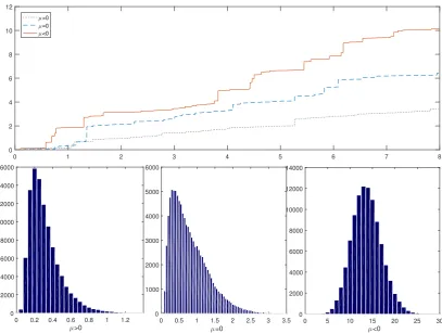
Figure 2.2:Comparison of the empirical CDF/PDF for SR scheme (via Algorithm2.4.6) ofSα,βwith the CDF/PDF obtained via numerical inverse using parameter settingsα=0.3, 0.6,β =1.0, 5.0, respectively.
For Algorithm2.4.6, the plots of CDFs and PDFs under parameter settingsα = 0.3, 0.6, β =
1.0, 5.0are provided in Figure2.2. We can see that our algorithm can achieve a very high level of
accuracy, the simulated CDFs and PDFs are fitted pretty well to the associated numerical inversions. There are a variety of available algorithms for numerically inverting Laplace transforms with high accuracy in the literature, such asGaver (1966),Stehfest(1970),Abate and Whitt (1992,1995, 2006) to name a few. Here, we adopt the classical Euler scheme as described inAbate and Whitt (2006, Section 5, p.415-416).
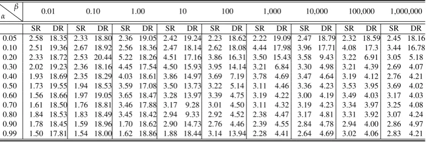
To investigate the performance of our SR scheme, we made a comparison of CPU time for Al-gorithm2.4.6against the DR scheme for simulating100, 000replications under parameter settings
α ∈ {0.05, 0.1, ..., 0.9, 0.99}andβ ∈ {0.01, 0.1, ..., 106}. The numerical results are reported in
Table2.1. We can see that our SR scheme performances well for all combinations ofαandβ. The
out-performance of our algorithm would even become much more substantial whenαis close to0.
For example, it is about8times faster than the DR scheme whenα=0.05. In addition, Algorithm
2.4.6is also very fast when the tilting parameter βis not very large, which clearly indicates that
Table 2.1:Comparison of CPU time for the SR scheme (via Algorithm2.4.6) against the DR scheme (
Dev-roye,2009) based on parameter settingsα∈ {0.05, 0.1, ..., 0.9, 0.99}andβ∈ {0.01, 0.1, ..., 106}; each value in the table is produced from100, 000replications.
α
β 0.01 0.10 1.00 10 100 1,000 10,000 100,000 1,000,000
SR DR SR DR SR DR SR DR SR DR SR DR SR DR SR DR SR DR
0.05 2.58 18.35 2.33 18.80 2.36 19.05 2.42 19.24 2.23 18.62 2.22 19.09 2.47 18.79 2.32 18.59 2.45 18.16 0.10 2.51 19.36 2.67 18.92 2.56 18.36 2.47 18.14 2.62 18.08 4.44 17.98 3.96 17.71 4.08 17.3 3.44 16.78 0.20 2.33 18.72 2.53 20.44 5.22 18.26 4.51 17.16 3.86 16.31 3.50 15.43 3.58 9.43 3.22 6.91 3.05 5.18 0.30 2.02 19.23 2.36 18.16 4.45 17.54 4.50 15.93 3.95 14.14 3.21 6.84 3.30 4.98 3.21 4.39 2.69 4.07 0.40 1.93 18.69 2.35 18.29 4.03 18.61 3.86 14.97 3.69 7.19 3.78 4.69 3.47 4.64 3.19 4.12 2.76 4.21 0.50 1.73 19.55 1.94 18.53 3.59 17.08 3.50 13.73 3.22 5.14 3.11 4.46 3.36 4.23 3.53 3.95 3.69 4.02 0.60 1.56 18.66 1.97 19.05 3.65 18.47 3.28 13.97 3.39 4.75 3.19 4.22 3.00 4.19 3.49 4.03 3.17 4.03 0.70 1.61 18.50 1.76 18.81 3.46 17.88 3.17 9.28 3.01 4.50 3.11 4.32 3.19 4.23 3.34 3.97 3.25 4.08 0.80 1.84 18.53 1.83 18.49 3.45 18.42 2.94 9.33 2.92 4.52 2.38 4.47 3.17 4.81 3.31 3.92 3.07 4.24 0.90 1.78 18.45 1.59 18.96 1.70 18.62 2.90 14.73 2.76 4.46 2.39 4.55 2.84 4.78 2.94 4.00 2.86 4.97 0.99 1.50 17.81 1.54 18.00 1.62 18.86 1.88 18.44 3.14 13.94 2.28 4.41 2.64 4.69 3.02 4.06 2.83 4.21
2.5
Conclusion
Chapter 3
Truncated Lévy Subordintors
In this chapter, we propose a new type of Lévy subordinators, namely the truncated Lévy subor-dinators, which is obtained by restricting the size of each jump. The truncated Lévy subordinator is defined through the Lévy measure with the limitation that the jump sizes do not exceed a certain truncation level. We study the path properties of truncated Lévy subordinator and develop exact simulation algorithm based on marked renewal process. In particular, we study several examples of truncated Lévy subordinators, such asthe Dickman process, the truncated gamma process, the truncated stable process, the truncated inverse Gaussian process, in details. This type of Lévy sub-ordinators has various applications in finance and insurance. First, we could use these processes to model aggregate claims distributions as individual claim sizes are often bounded from above. We also discover that the value of truncated Lévy subordinator at timetis the value of a perpetuity
with stochastic discounting. Besides, we observe that the process has a duality relationship with the Parisian stopping time of diffusion processes. Hence our algorithms provide alternative methods for pricing Parisian options and bonds.
3.1
Preliminaries
Definition 3.1.1. A truncated Lévy subordinatorZtis defined by restringing the Lévy measureν
with an upper boundb. The Laplace transform ofZtis given as
Eî
e−vZtó=exp
Ö
−t
b
Z
0
(1−e−vz)ν(z)dz
è
, v∈R+.
Zt preserves most properties of the original Lévy subordinator. It is a non-decreasing process
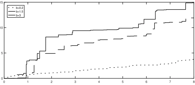
to exceed a certain levelb. This is illustrated in Figure3.1, where we plot the sample paths of a
truncated Lévy subordinatorZtfor three different truncation levelsb.
0 1 2 3 4 5 6 7 8
0 5 10 15
[image:36.595.95.502.123.301.2]b=0.2 b=1.5 b=3
Figure 3.1:Sample paths of a truncated Lévy Subordinator withb=0.2, 1.5, 3, respectively.
The original non-truncated Lévy subordinatorXtis thus equivalent to
Xt=DZt+Rt,
whereZt is the truncated Lévy subordinator with Lévy measure restricted to(0,b), and Rt is a
compound Poisson process with meant
Z ∞
b
ν(x)dx, independent fromZt, and the density of its
jump sizes is
f(x) = Z ∞ν(x)
b ν
(x)dx
, b≤x< ∞.
This allows us to consider subordinators whose Lévy measure is discontinuous atb, and thus jump
sizes are not characterised by a single continuous distribution. More generally,Rtcan be replaced
by any compound Poisson process with an arbitrary Poisson rate and jump distribution.
The paths of the truncated Lévy subordinatorZt can be characterised via hitting times and
as-sociated overshoots. The definitions for hitting time and corresponding overshoot are provided as below,
Definition 3.1.2. LetTbe the first hitting time of levelbof the truncated Lévy subordinatorZt,
andW be the associated overshoot at timeT, i.e.
T : = inf{t>0|Zt >b}, (3.1.1)
3.2
Distributional Properties
The general representation of the joint distribution of the first passage time and the associated overshoot is formulated in Theorem3.2.1.
Theorem 3.2.1. LetTbe the first hitting time of levelbofZtwith Lévy measureν, andW be the
overshoot at timeT. Then the joint distribution of(T,W)is given by
fT,W(t,w) = b
Z
w
f(y,t)ν(b+w−y)dy, (3.2.1)
wheret ∈(0,∞),w∈(0,b), and f(·,t)denotes the density ofZtwithin(0,b). In particular, we
have
f(·,t) =eν¯(b)tf
Xt(·,t)1{0<x<b}, (3.2.2)
whereν¯(s):=
∞
Z
s
ν(x)dx, and fXt(·,t)is the density ofXtwith Laplace transform
Eî
e−vXtó=exp
Ñ −t ∞ Z 0 Ä
1−e−vxäν(x)dx
é
. (3.2.3)
Proof. Using the strong Markov property of Lévy processes, we have
P(T∈dt,W >w) = lim
e→0
1
eP(Zt−e≤b,Zt
>b+w)
= lim e→0 1 e b Z 0
P(Zt−e∈dy)P(Ze>b+w−y)
=
b
Z
0
f(y,t)
∞
Z
b+w−y
ν(u)dudy, (3.2.4)
Differentiating (3.2.4) with respect tow, the joint density of(T,W)directly follows (3.2.1). The density ofZtwithin(0,b)can be derived though its Laplace transform, we have
f(x,t) = L−1¶ Eî
e−vZtó©1
{0<x<b}
= L−1
exp Ñ −t ∞ Z 0 Ä
1−e−vxäν(x)dx
é exp Ñ t ∞ Z b Ä
1−e−vxäν(x)dx
é
1{0<x<b}
= L−1
exp Ñ −t ∞ Z 0 Ä
1−e−vxäν(x)dx
é exp Ñ t ∞ Z b
ν(x)dx
é exp Ñ −t ∞ Z b
e−vxν(x)dx
é
= L−1
∞
Z
0
e−vxfXt(x,t)dxexp
Ñ
t ∞
Z
b
ν(x)dx
é
∞
X
k=0
(−t)k
k!
Ñ ∞
Z
b
e−vsν(x)dx
ék
1{0<x<b}
= eν¯(b)tf
Xt(x,t)1{0<x<b}.
where fXt(·,t)denotes the density ofXtwith Laplace transform (3.2.3).
Under the circumstance that the first passage time of Zt hits levelbis greater thant, the
dis-tribution of the truncated processZtis characterised via its density within (0,b). The details are
illustrated in Theorem3.2.2.
Theorem 3.2.2. Given the timet, the density of{Zt|Zt <b}is given by
fZt|Zt<b(x|t) =
fXt(x,t)
b
Z
0
fXt(x,t)dx
, 0<x <b, (3.2.5)
wherefXt(·,t)denotes the density ofXtwith Laplace transform(3.2.3).
Proof. The density immediately follows (3.2.5) by truncating the density ofXt.
3.3
Marked Renewal Representation
The paths of the truncated subordinatorZtcan be characterised by a marked renewal process. First,
we define a sequence of hitting timesT1,T2,T3, ...,and denotingSi = i
P
j=1
Tj, let
Ti :=inf{t> Si−1|Zt > ZSi−1 +b}, i=2, 3, ..., (3.3.1)
TheseT1,T2, ...are treated as the holding times for the events{Ti−1 < t < Ti|Zt−ZTi−1 < b}, fori=2, 3, .... We further defineW1,W2, ...to be the overshoots at timeS1,S2, ..., i.e.
Wi := ZSi −ZSi−1−b. (3.3.2)
Hence, at timeSi the process will automatically increase by(b+Wi)units for all i. Since the
processZthas independent and stationary increments, each pair of(Ti,Wi)are independent and
identically distributed with joint density given in Theorem3.2.1. In addition,Wi will be bounded
by0andbfor allias the jump sizes of the process is restricted with an upper boundb. The value
of the process at timeSn will be ZSn =
n
P
i=1
therefore can be expressed as using a marked renewal process as follows,
Zt = Nt
X
i=1
(b+Wi) +
Ä
Zt−ZSNt |SNt <t< SNt+Tn+1;Zt−ZSNt <b+Wn+1
ä
, (3.3.3)
whereNt =
∞
P
i=11{Si≤t} is determined via (3.3.1) such thatt
[image:39.595.94.541.244.582.2]∈ [SNt,SNt +Tn+1). We also use Figure3.2to illustrate the marked renewal idea graphically. The first part in (3.3.3) represents the
Figure 3.2:Graphical illustration of a sample path ofXt
T1
b
b b+W1
T1+T2
2b+W1
2b+ P2
i=1
Wi
3b+ P2
i=1Wi
b
T1+T2+T3 T1+...+Tn T1+...+Tn+1
ZSNt
nb+n−1P
i=1
Wi
nb+ Pn
i=1
Wi
t Zt
nb+b+ Pn
i=1Wi
nb+b+nP+1
i=1
Wi
b+Wn+1
time
position of the truncated process at timeSNtbefore reachest. The second term in (3.3.3) represents the movement of the process within the timet−SNt. As{t−SNt <Tn+1}
D
={Zt−SNt <b}, we
have
{Zt−ZSNt |SNt <t<SNt+Tn+1,Zt−ZSNt <b+Wn+1}
D
= {Zt−SNt|t−SNt < Tn+1,Zt−SNt <b+Wn+1}
D
= {Zt−SNt|Zt−SNt <b,Zt−SNt <b+Wn+1} D
Conditioning ont−SNt < Tn+1 and Zt−SNt < b+Wn+1, the distribution of Zt−SNt satisfies (3.2.5) in Theorem3.2.2. Thus,Ztcan be simulated by generating pairs of hitting time and
over-shoot(Ti,Wi), stopping when the sum of Ti that have been generated, saySNt+Tn+1, becomes larger than the inputt. We then generate the part{Zt−SNt|Zt−SNt < b}and return to (3.3.3). We
give the details of the exact simulation method in Algorithm3.3.1. In particular, we show how to emphasis the marked renewal procedure using a recursive loop.
Algorithm 3.3.1(Marked Renewal Simulation Framework). The truncated Lévy subordinatorZt
can be simulated via the following steps:
1. SetS =0,
2. Generate(T,W)from the distribution fT,W(t,w)in(3.2.1); Ift < T, go to step 3;
Other-wise, go