Mitigating Noise in Interferometric Gravitational Wave
Detectors
Thesis by
William Zachary Korth
In Partial Fulfillment of the Requirements for the
Degree of
Doctor of Philosophy
CALIFORNIA INSTITUTE OF TECHNOLOGY
Pasadena, California
2019
ii
© 2019
William Zachary Korth ORCID: 0000-0002-4422-1070
ACKNOWLEDGEMENTS
I have spent well over a third of my life in LIGO. It has been a long road, and one
that’s been as challenging as it has been rewarding. Over my years in graduate
school, I can barely count the number of choices I made that prolonged the journey
significantly. I regret none of them.
To Guido, Dave R. and Dave T., thank you for bringing me into this remarkable
family, and for giving me the opportunity to be a part of something truly great.
To Eric B. and Ken, thanks for initiating me into the LIGO Lab and for an
unforget-table summer at Caltech.
To Rana, thank you for believing that I had what it takes and for helping me remember
when I forgot. You have been an inspiration to me from the beginning, as you are
to so many others. It has been a privilege to work under you.
To Alan, Yanbei and Keith, thank you for your unwavering support through thick
and thin. I could not have asked for a better committee. Also to Alan and Yanbei,
thank you for all you have taught me, whether in a classroom or over a beer or three.
To Julie, Tess and Sofie, thank you for all your help with every form, deadline and
submission over the years.
To Eric G., thank you for always having my back and for letting some of those
regular reports slide. I will miss stopping by your office to talk about whatever
strikes our fancy.
To Aidan, Alastair, Dmass, Jenne, Frank, Jan, Gabriele, Jamie, Nic, Chris W.,
Larry, Rory, Tara, Matt, Alberto, Andrew, Kiwamu, Jeff K., and everyone who
came before me, thank you for all you’ve taught me; I will always cherish the time
we spent together. To Eric, Evan, Den and those who came after me but still somehow got out before me, I forgive you!
To Aaron, Brittany and Johannes, thanks for sharing the Cryo lab with me for these
past couple years, and for all your help in finally getting me out of it! To Gautam
and Craig, it was a pleasure sharing a softball championship with you.
To Valera, Ryan, Chris M., Anamaria, Jan, Keiko, Adam, Den, Suresh, and the rest
of the Swamp Donkeys, I think you already know how I felt about leaving Louisiana;
iv
a half or so among the best of my life. To Thomas, thanks for letting me crash your
lab for a while and for teaching me a great deal.
To Haixing, thank you for the countless hours we spent talking about quantum noise
and about life. I will always be moved by your intellect and your philosophy.
To Rich, thanks for teaching me damn near all I know about electronics. I am forever
grateful for the number of afternoons you spent with me at your whiteboard after I
showed up unannounced. Thanks, too, for all the parts I pilfered from the Downs
lab over the years.
To Koji, thank you for the sheer amount of knowledge, intuition, and general
ex-perimental wisdom you have bestowed upon me over the years. I would not be the
person I am today without the constant support and guidance you have given me
from my first day to my last.
To Ernie, thank you for feeding me! By my count, I probably visited your magical
truck of deliciousness over 2000 times. Don’t think for a second I won’t be making
occasional Thursday trips back to Pasadena just for a spicy beef fix!
To my beautiful wife, Gretchen, thank you for dragging me into an unheated pool
in the dead of winter, then down a mountain, then out a perfectly good plane and
into your life forever. Thanks for hopping in a car a few days after your defense
and driving across the country to a new home, sight-unseen. Thanks for always
believing in me and for everything you’ve done to get us where we are today. I can’t
wait to see where our next adventure takes us. I love you.
To my little Max, thanks for playing your own tiny part to make sure this thesis was
finished in under a decade. We’ve only just met you, but you’ve already brought us
so much joy. I love you, too.
To Tiny, Mufasa, Scotty, Peeps, Dory and Frankie, thanks for occasionally taking
time out of your day—and mine—to remind me that sometimes snuggles are more
important than really getting much of anything done.
Last but not least, to my incredibly loving family, thank you for making me the man
I am. Thank you for giving me the tools I needed to succeed in this world, and the
will to do it. I love you all so very much.
To the many people I’m sure to have forgotten here, thank you for being a part of
ABSTRACT
Gravitational waves, first predicted by Einstein in 1916, eluded detection for nearly a
century. These faint ripples in the fabric of spacetime, with typical strain amplitudes
at the Earth on the order of |h| ∼ 10−22, carry secrets of the universe untold by electromagnetic radiation. Following decades of research and development, a
network of terrestrial interferometric detectors succeeded in measuring the passing
of a gravitational wave (GW150914) for the first time in 2015. Individual detectors
within this network are currently said to be operating in a “second-generation”
configuration; over the next decade, planned upgrades will take these detectors
beyond this into a new generation. This thesis concerns the characterization and
reduction of noise in one of these second-generation detectors, Advanced LIGO, as
well as efforts underway to improve its sensitivity in the coming years.
The first part of this thesis is a detailed overview of gravitational waves, the history of
gravitational wave detection, and a reasonably thorough description of the Advanced
LIGO detector. Particular attention is paid to a pedagogical motivation of the optical
configuration of Advanced LIGO with reference to its forebears. This part ends with
an overview of the sources of noise limiting the sensitivity of Advanced LIGO, and
an exposition of plans to reduce their influence in the future.
The second part describes the development of a laser gyroscope for use in tilt sensing
in Advanced LIGO, starting with a motivation of the work based on limitations in
the area of seismic noise sensing and cancellation.
The third part recounts the design, fabrication, testing, installation and
commission-ing of an important component of the Advanced LIGO detector: the output mode
cleaner (OMC).
The fourth part outlines a proposed scheme for reduction of quantum noise in
gravitational wave detectors and other experiments. In particular, this scheme
allows for the operation of a so-called “optical spring” cavity in such a way as to be
largely immune from the deleterious effects of quantum radiation pressure noise.
The fifth and final part describes progress towards a direct measurement of thermal
noise in thin silicon ribbons, which is pertinent to the design of suspensions in future
cryogenic gravitational wave detectors.
vi
PUBLISHED CONTENT AND CONTRIBUTIONS
Korth, W. Z., A. Heptonstall, E. D. Hall, K. Arai, E. K. Gustafson, and R. X. Adhikari (2016). “Passive, free-space heterodyne laser gyroscope”. In:
Clas-sical and Quantum Gravity33 035004. doi: https://doi.org/10.1088/
0264-9381/33/3/035004.
W.Z.K. participated in the conception of the experiment, conducted it, and wrote the paper.
Korth, W. Z., H. Miao, T. Corbitt, G. D. Cole, Y. Chen, and R. X. Adhikari (2013). “Suppression of quantum-radiation-pressure noise in an optical spring”. In:
Physical Review A88033805. doi: https://doi.org/10.1103/PhysRevA.
88.033805.
TABLE OF CONTENTS
Acknowledgements . . . iii
Abstract . . . v
Published Content and Contributions . . . vi
Table of Contents . . . vii
List of Illustrations . . . xi
List of Tables . . . xv
I
Background and Theory
1
Chapter I: Gravitational waves . . . 21.1 Basic gravitational wave theory . . . 2
1.1.1 General relativity . . . 2
1.1.2 Gravitational waves . . . 3
1.2 History of detection science . . . 6
1.2.1 First estimates: Hertz-type experiment . . . 6
1.2.2 Early detection attempts: Weber’s resonant bars . . . 7
1.2.3 Astronomical observations . . . 8
1.2.4 Laser interferometers . . . 9
Chapter II: State of the art: Advanced LIGO . . . 11
2.1 Description of the instrument . . . 11
2.1.1 Optical configuration . . . 11
2.1.2 Systems and control. . . 29
2.2 Noise . . . 38
2.2.1 Seismic and gravity-gradient (Newtonian) noise . . . 39
2.2.2 Laser noise . . . 40
2.2.3 Scattered light noise . . . 41
2.2.4 Residual gas noise . . . 41
2.2.5 Electronic noise . . . 42
2.2.6 Quantum noise . . . 42
2.2.7 Thermal noise . . . 45
2.3 The path forward . . . 46
2.3.1 Reducing noise in LIGO upgrades . . . 46
2.3.2 Putting it all together: the case for silicon in LIGO Voyager . 49 2.3.3 Outstanding questions about silicon . . . 50
II
Laser Gyroscope
52
Chapter III: Tilt sensing in Advanced LIGO . . . 54viii
4.1 Introduction . . . 57
4.1.1 Laser gyroscopes . . . 57
4.1.2 Current laser gyroscope sensitivities . . . 58
4.1.3 Rotation sensing . . . 59
4.2 The passive, free-space laser gyroscope . . . 60
4.2.1 Overview . . . 60
4.2.2 Detailed experimental design . . . 62
4.2.3 Realized performance and noise analysis . . . 65
4.3 Possible future designs . . . 72
4.4 Conclusion . . . 73
III Advanced LIGO Output Mode Cleaner
75
Chapter V: Background . . . 765.1 DC Readout . . . 76
5.2 Mode cleaners in detail . . . 77
5.2.1 Transverse modes and Gaussian beams . . . 77
5.2.2 Cavity transverse mode spacing and higher-order mode trans-mission spectrum . . . 80
Chapter VI: The Advanced LIGO OMC . . . 84
6.1 Optical design . . . 84
6.2 Mechanical design, fabrication and benchtop testing . . . 86
6.2.1 Overall construction and components . . . 86
6.2.2 Mirror characterization and bench assembly . . . 91
6.3 Installation . . . 93
6.3.1 OMC suspension assembly . . . 93
6.3.2 Detector electronics . . . 94
6.4 Integration . . . 98
6.4.1 Bring-up. . . 98
6.4.2 Control system . . . 99
6.4.3 Advanced LIGO commissioning with the OMC . . . 103
IV Suppression of Quantum Radiation Pressure Noise in
an Optical Spring
107
Chapter VII: Suppression of Quantum Radiation Pressure Noise in an Optical Spring . . . 1097.1 Introduction . . . 109
7.2 Optical spring . . . 111
7.3 Evading quantum radiation pressure noise . . . 113
7.4 Residual radiation pressure noise . . . 114
7.5 Experimental realization with double optical spring . . . 116
V
Thermal Noise in Silicon Ribbons
119
Chapter VIII: Thermal noise theory, resonator design, and numerical modeling1218.1 Thermal noise in detail . . . 121
8.1.1 The loss angle . . . 121
8.1.2 The fluctuation-dissipation theorem (again) . . . 123
8.1.3 Sources of loss . . . 123
8.2 Suspension thermal noise in LIGO Voyager . . . 126
8.2.1 Background . . . 127
8.2.2 The ribbon cross section . . . 127
8.2.3 Suspension thermal noise . . . 127
8.2.4 Conclusion . . . 131
8.3 Ribbon cantilever design and numerical modeling . . . 132
8.3.1 Design. . . 132
8.3.2 Finite-element analysis (FEA) numerical model . . . 134
Chapter IX: Cantilever fabrication . . . 138
9.1 Fabrication process. . . 138
9.1.1 Overview . . . 138
9.1.2 Detailed recipe . . . 138
Chapter X: Characterizing loss: Ringdown measurements . . . 148
10.1 The apparatus . . . 148
10.1.1 The clamp . . . 148
10.1.2 The cryostat . . . 149
10.2 Operation . . . 150
10.2.1 Thermal control . . . 150
10.2.2 Resonator readout and control . . . 152
10.3 Measurements . . . 155
10.3.1 Expectations . . . 155
10.3.2 Results . . . 156
10.3.3 Analysis . . . 157
Chapter XI: Interferometric interrogation of cantilever displacement noise . . 159
11.1 Overview . . . 159
11.1.1 Design. . . 159
11.1.2 Target sensitivity . . . 161
11.2 Detailed description . . . 162
11.2.1 Optical system . . . 162
11.2.2 Physical system . . . 164
11.2.3 Electrical system . . . 167
11.3 Experimental progress . . . 169
11.3.1 Phase I: Test cavities . . . 169
11.3.2 Phase II: Dummy cantilever cavities . . . 173
11.3.3 Phase III: Real cantilever cavities . . . 181
11.4 Conclusion . . . 184
Bibliography . . . 187
Appendix A: Feedback control . . . 203
x
A.2 Stability . . . 206
Appendix B: Pound-Drever-Hall locking . . . 207
Appendix C: Supplemental optical spring radiation pressure noise calculations210
C.0.1 Ideal situation—no optical loss and leading-order terms . . . 210
C.1 Realistic situation—optical loss and next-order corrections . . . 214
C.2 Feedback and closed-loop response . . . 216
LIST OF ILLUSTRATIONS
Number Page
1.1 The two orthogonal gravitational wave polarization modes . . . 5
2.1 Illustration of a gravitational wave’s effect on the orthogonal arms of a Michelson interferometer. . . 13
2.2 A Michelson interferometer with Fabry-Pérot arm cavities. . . 15
2.3 Diagram of a Fabry-Pérot cavity. . . 16
2.4 A Michelson interferometer with Fabry-Pérot arm cavities and power recycling. . . 19
2.5 Transfer function from input laser power noise to apparent GW signal in a PRFPMI . . . 25
2.6 Effective model for the common-mode coupled cavity. . . 25
2.7 The full core aLIGO optical configuration . . . 27
2.8 More accurate diagram of the aLIGO optical layout. . . 30
2.9 Simple block diagram of a typical digital control loop in aLIGO. . . . 31
2.10 Advanced LIGO PSL. . . 33
2.11 Advanced LIGO seismic isolation system. . . 34
2.12 A simple, single-stage pendulum. . . 35
2.13 Detail of the Advanced LIGO quadruple suspension. . . 37
2.14 Advanced LIGO noise budget. . . 38
2.15 Quantum noise spectral density. . . 44
2.16 Squeezed states. . . 48
2.17 Coefficient of thermal expansion (CTE) of monocrystalline silicon. . 50
3.1 Simplified demonstration of the seismometer tilt-coupling problem. . 55
3.2 The aLIGO tilt-sensing requirement definition. . . 56
4.1 Performance for a number of different rotation sensors. . . 61
4.2 Simplified diagram of the laser gyroscope. . . 62
4.3 Photo of the laser gyroscope experiment. . . 63
4.4 Noise budget of the laser gyroscope. . . 65
4.5 Diagram of the out-of-loop RAM monitor setup. . . 72
4.6 Proposed fiber-distributed gyroscope array scheme. . . 72
5.1 Diagram of a Gaussian beam. . . 78
xii
6.1 HOM spectrum for a cavity with the coarse parameters chosen for
the OMC. . . 85
6.2 Power-law models of the eLIGO dark port field spatial structure. . . . 87
6.3 Simulated length scan of the OMC. . . 88
6.4 Simulated radius of curvature scan of the OMC. . . 88
6.5 As-built diagram of the L1 OMC. . . 89
6.6 Diagram of the OMC mirror curvature measurement setup. . . 91
6.7 Diagram of the OMC test setup. . . 93
6.8 Photo of the interior of HAM6. . . 95
6.9 Bird’s-eye diagram of the HAM6 layout. . . 96
6.10 Evaluation of the input-referred noise of the in-vacuum DCPD preamps. 97 6.11 Evaluation of the voltage transfer function of the in-vacuum DCPD preamps. . . 98
6.12 Simple diagram of the digital model for the OMC length and angular control. . . 100
6.13 OMC control screen. . . 101
6.14 Dither locking diagram. . . 102
6.15 Length scan of the OMC while closely aligned to the interferometer output beam. . . 104
6.16 Noise in the low-noise power-recycled Michelson interferometer (PRMI) during aLIGO commissioning. . . 106
7.1 Simplified experimental layout. . . 112
8.1 A simple mass-spring system with damping. . . 121
8.2 Illustration of the thermoelastic loss mechanism. . . 124
8.3 Possible LIGO Voyager suspension ribbon cross sections. . . 127
8.4 Projection of LIGO Voyager suspension thermal noise as a function of ribbon aspect ratio. . . 129
8.5 Normalized strain energy density along the bending direction of a ribbon. . . 131
8.6 Total loss factor as a function of surface layer loss and thickness, for the two extremal aspect ratios. In each case, the acceptable total loss contour is highlighted in green. . . 132
8.7 Design of the silicon cantilever. . . 133
8.8 The first few cantilever mode shapes. . . 134
8.9 Cantilever mechanical transfer function. . . 136
9.1 Cantilever fabrication process. . . 139
9.2 Wafer before and after PECVD nitride deposition. . . 141
9.3 Demonstration of the operation of the contact aligner for photolithog-raphy. . . 142
9.4 Mask for the photolithography process. . . 143
9.5 Demonstration of the appearance and transfer of the photolithography pattern during development and dry etching. . . 143
9.6 The KOH through-etch. . . 145
9.7 The second round of etching.. . . 146
10.1 Stainless steel clamp used to hold the cantilever. . . 149
10.2 Clamp alignment jig. . . 150
10.3 Photo of the ringdown measurement experimental volume. . . 151
10.4 Control screen of the mode ringer module. . . 153
10.5 Calculated thermoelastic loss vs. temperature for the cantilevers. . . . 156
10.6 Typical ringdown measurement results. . . 157
11.1 Optical layout for the interferometric experiment. . . 160
11.2 Initial noise budget estimate for the interferometric experiment. . . . 161
11.3 Drawing of the cryostat used to hold the ribbon cantilever cavities. . . 165
11.4 Diagram of the suspension from which the optical breadboard is hung within the cryostat. . . 166
11.5 Modal analysis of the suspension. . . 167
11.6 Two electronic chains used in the differential cavity beat note readout. 168 11.7 Test cavities. . . 170
11.8 Evolution of the beat spectrum over part of the test cavity phase. . . . 171
11.9 Detailed FEA model of the test cavity payload. . . 172
11.10 Test cavity mode identification. . . 173
11.11 Inter-experiment beat measurement. . . 174
11.12 Optical contacting of the mirrors to the cantilevers. . . 175
11.13 Demonstration of the adapter piece between the cantilever clamps and the suspended breadboard. . . 176
11.14 Demonstration of the radiation pressure cantilever actuation. . . 178
11.15 In-situ cantilever ringdown using radiation pressure excitation. . . 179
xiv
11.17 Comparison of the mechanical responses of the dummy and real
cantilevers. . . 181
11.18 Monolithic suspended payload design. . . 182
11.19 Comparison of the measured noise in the real and dummy cantilever
cases, with thermal noise estimates. . . 183
11.20 Attempt to explain the elevated noise level using anomalously low-Q
higher-order bending modes. . . 185
A.1 Diagram of a generic feedback loop. . . 204
B.1 A Pound-Drever-Hall locking setup. . . 207
C.1 A graphical representation of the feedback model described in the text.217
LIST OF TABLES
Number Page
2.1 Definitions of the five interferometer length degrees of freedom. . . . 37
7.1 A sample set of parameters. These values generate an optical spring
with ωos/2π ≈ 100 kHz andQeff ≈ 109. The laser powers PB and
PR refer to the circulating powers, andQ refers to the quality of the
bare mechanical system. For the specified geometry, the required
finesses are of orderF ≈10,000, compatible with the optical quality of resonators in production today. . . 117
8.1 Parameters used for the LIGO Voyager suspension thermal noise
calculation. . . 129
8.2 Acceptable total loss for each aspect ratio option in the LIGO Voyager
Part I
Background and Theory
C h a p t e r 1
GRAVITATIONAL WAVES
1.1 Basic gravitational wave theory
Here, I will give averybrief summary of general relativity and gravitational waves.
1.1.1 General relativity
Gravity, a fundamental force of nature, is currently best understood using Einstein’s
theory of general relativity (GR) [1]. In contrast to the earlier Newtonian theory,
which treated the force of gravity as an instantaneous attractive interaction between
any two massive objects, general relativity describes the phenomenon as arising from
the interaction of matter and energy with the continuum of spacetime. Specifically,
the presence of matter or energy induces a local curvature in the spacetime manifold, which in turn affects the trajectories of objects through it.1
In this way, the effect of gravity can be understood as a purely geometrical one:
ob-jects under the sole influence of gravity must travel along an extremal 4-dimensional
(4-D) path—known as a geodesic—that is determined everywhere by the local spacetime curvature.
General relativity is therefore a field theory of gravity, governed by the Einstein
field equation2:
Gµν = 8πG
c4 Tµν. (1.1)
On the right-hand side of this equation,Gis Newton’s gravitational constant,cis the
speed of light in vacuum, andTµν, known as the stress-energy tensor, represents matter and energy present in a region of spacetime. The quantity on the
left-hand side,Gµν, is called the Einstein tensor, and it encapsulates the curvature of spacetime. More concretely, the Einstein tensor is constructed as
Gµν = Rµν− 1
2
gµνR. (1.2)
Here, the quantities Rµν and R, known as the Ricci tensor and the Ricci scalar, respectively, are both derived by contraction of a higher-rank tensor,Rρσµν, termed
1In the words of Misner, et al. [2], “spacetime tells matter how to move; matter tells spacetime
how to curve.”
2This equation and ones that follow in this chapter contain tensors. The reader should be familiar
3
theRiemann curvature tensor:
Rµν = Rλµλν (1.3)
R = Rλλ. (1.4)
The quantitygµν, called themetric tensor(or simply “the metric”), directly encodes the geometry of spacetime and appears in GR whenever this geometry is invoked.
For example, the metric is used when calculating tensor contractions (e.g., R =
Rλλ = gµνRµν)3. It is also used in the definition of the Riemann curvature tensor,
Rρσµν = ∂∂
xµΓ
ρ
νσ− ∂∂
xνΓ
ρ
µσ +ΓρµλΓλνσ−ΓρνλΓλµσ, (1.5)
via theChristoffel symbols:
Γλµν = 1
2
gλ ρ ∂gρµ ∂xν +
∂gρν ∂xµ −
∂gµν ∂xρ
!
. (1.6)
Most pointedly, the metric determines thespacetime interval(orline element),
ds2= gµνxµxν, (1.7)
which generalizes the concept of distance in three dimensions to 4-D. By extremizing
an action defined as the length of a curve in spacetime (i.e., S =
R
ds), one arrives
at thegeodesic equation:
d2xµ dτ2 +
Γµρσdx
ρ
dτ dxσ
dτ =0, (1.8)
where the proper timeτis defined with respect to the spacetime interval as
dτ2 ≡ −ds2 . (1.9)
1.1.2 Gravitational waves
In regions far from any matter or energy, we have Tµν ≈ 0. Here, defining the
Minkowski metricthat describes flat spacetime,
ηµν = * . . . . . . ,
−1 0 0 0
0 1 0 0
0 0 1 0
0 0 0 1
+ / / / / / / -, (1.10)
3The quantitygµνfound here is known as theinverse metric tensorand is defined through the
we can write
gµν = ηµν+hµν (1.11)
and treat spacetime as flat, save for a small perturbation hµν, called the spacetime
strain. In this regime, known as theweak-field limit, one can search for solutions
to a wave equation inhµν of the form [2]
∇2− 1 c2
∂2
∂t2
!
hµν = 0. (1.12)
After appropriate gauge fixing4, a solution to this equation can be found of the form
hµν(t,z) =
* . . . . . . ,
0 0 0 0
0 h+ h× 0
0 h× −h+ 0
0 0 0 0
+ / / / / / / -cos f ωGW
t− zcg , (1.13)
where the orthogonal polarization amplitudesh+andh×are known as “h-plus” and “h-cross”, respectively. This equation describes a gravitational wave of angular
frequencyωGWtraveling in the+zˆdirection.
Using (1.7), (1.11) and the form ofhµνwe can see that, att,z =0 in the presence of
this perturbation, the line element becomes
ds2 =−c2dt2+(1+h+)dx2+(1−h+)dy2+2h×dxdy+dz2 . (1.14)
Apparently, spacetime has beenstretchedin the ˆxdirection andcompressedin the ˆy direction by the factor
√
1+h+ ≈ (1+ h2+). Due to the oscillatory nature of (1.13), it is clear that the opposite will be true at a GW phase shift ofπfrom this point. The
orthogonal polarization amplitude h× has the identical effect, only along the lines
y = xand y = −x, as can be confirmed by a coordinate rotation of 45◦about thez
axis. These polarizations can be combined with an arbitrary phase shift to produce
more complicated waveforms (e.g., “circularly polarized” GWs, etc.). A diagram
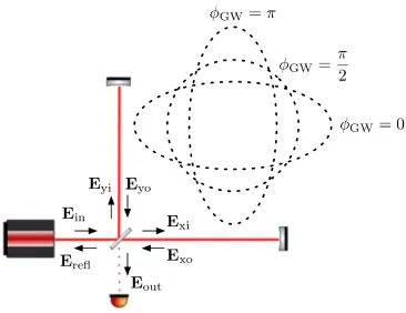
of these modes can be found in Fig.1.1.
1.1.2.1 GW sources and amplitudes
Gravitational waves are generated by any object with a fluctuating quadrupole
moment. Given a source object A with quadrupole moment Iµν(A), the spacetime
4The choice of gauge used here, called the transverse traceless (TT) gauge, assigns fixed
5
GW : 0
⇡ 2
3⇡ 2
⇡ 2⇡
h+
h⇥ x
[image:20.612.116.506.82.321.2]y
Figure 1.1: The two orthogonal gravitational wave polarization modes, h+ andh×, as a function of phase. It should be easy visualize the “circular polarization” that results from a combination of these two with a phase shift ofπ/2.
strain caused by A evaluated a distancer away is given by [3]
h(µνA)(r,t) = 2G
rc4I¨
(A)
µν (t− rc), (1.15)
where the dots denote time derivatives.
How large are gravitational waves? By definition, the strain amplitudes are far
smaller than unity (h≡ |hµν| 1), but by how much? As I’ll show in more detail
in Sec. 1.2.1, we can use (1.15) to estimate the amplitude of a GW reaching the
earth from some hypothetical source. For instance, a binary star system located 30
Mpc away, whose constituents are two solar-mass neutron stars orbiting one another
nearly close enough to touch (on the order of 10 km), would produce a peak strain
on earth of h ≈ 10−21! Due to their extreme faintness, then, GWs from all but the most violent events in the universe bear no hope of being detected here on earth.
Gravitational wave sources can be roughly divided into four categories:
• Continuous: Steady sinusoidal signals produced by individual rotating mas-sive objects (e.g., a neutron star with a mountain on its surface).
• Burst: Brief, wideband signals theoretically emitted by some energetic ob-jects like supernovae.
• Stochastic: Cosmic background produced by phase changes in the early universe.
To date, all GW detections have been in the compact binary inspiral category.
1.2 History of detection science
Even as he first predicted them, Einstein was already thinking about the possibility
of detecting gravitational waves [4]. Given how hard they would be to measure,
however, he himself had little confidence we would ever do so. It took a number of
years for the scientific community to reach a consensus that the GWs were real and
produced an observable effect [5].
1.2.1 First estimates: Hertz-type experiment
In 1879, the Berlin Academy of Sciences offered a prize to anyone who could prove
experimentally the relationship between electromagnetic forces and the dielectric
polarization of insulators. Heinrich Hertz pursued this prize at the insistence of
his mentor, Hermann von Helmholtz [6]. In a series of experiments throughout the
1880s, Hertz built scientific apparatuses to generate electromagnetic waves and then
detect them, all within the same laboratory. In doing so, he experimentally confirmed
many of James Clerk Maxwell’s theoretical predictions on electromagnetism.
Given the clear parallels, one might ask if it is possible to perform the analogous
experiment with GWs. For example, if we took a barbell-like object with heavy
masses on either end and then rotated it rapidly, what would be the magnitude of
the GWs generated? Following the analysis in [3], we can use (1.15) to answer that
question.
The quadrupole moment is defined as
Iµν ≡
Z
(xµxν− 1 3δµνr
2)ρ(r)
dV . (1.16)
If we assume our radiator is a barbell of point mass M on each side, separated by
7
plane, this gives5:
Ix x = M d 2
2
f
cos2(2πfrott)− 13
g
(1.17)
Iy y =
M d2
2
f
sin2(2πfrott)− 13
g
(1.18)
Ixy = Iyx =
M d2
2 cos(2πfrott)sin(2πfrott). (1.19) Therefore, using (1.15):
h= |hµν| ∼ 8π
2G c4
M d2f2 rot
z , (1.20)
wherezis the distance from the x−yplane at which we make our detection. Let’s
say we could manage to make a device with M = 1000 kg, d = 1 m, and frot = 1
kHz. That would give
h∼ 6.5×10−34× 1 m z
!
. (1.21)
As if that weren’t bad enough, in order to distinguish a GW from near-field effects,
we would need to be far from the source in thewave zone(i.e., z & λGW = 2
πc
ωGW). Even at the nearer edge withz = λGW≈ 300 km, this gives
hbest∼ 2×10−39,
(1.22)
which is very, very small.
1.2.2 Early detection attempts: Weber’s resonant bars
As it was clear that the only gravitational waves we would stand a chance of detecting
would be astrophysical in origin, experimenters started devising apparatuses to make
such a measurement. In the 1960s, Joseph Weber began searching for GWs with large
aluminum cylinders [7], which he realized could be used as mechanical resonant
amplifiers.
To understand how bar detectors work, it helps to introduce the concept of treating
a GW as a tidal force acting on the detector system. Imagine two free point masses
of mass M separated in space by a distance L. If a GW were to act on these
masses with strain amplitudeh(t)along the line between them, then—relative to the midpoint between them—an experimenter would see that each object is displaced
by a distance
xGW(t) = L
2
h(t)
2 . (1.23)
5Thezcomponents ofIµνeither vanish or are constant, and therefore do not contribute to GW
Given this displacement response, one can write down an apparent gravitational
wave force of magnitude
|FGW| ≡Mx¨GW = M L
4 ¨
h (1.24)
acting on each object.
Even though the calculation above is done for two free masses, it would still be valid
to useFGWto describe the passing GW even if we were to connect the two masses
using a spring. In that case, we would expect the system’s response to GWs,x/h, to
be augmented by the resonant mechanical response of the system to external forces.
In fact, this force approach can be used to calculate the effect of a passing GW on an arbitrarily constructed distribution of mass6. Taking advantage of this effect,
one can use high-quality mechanical resonators as bells, ringing at their resonant
frequencies when acted upon even by the paltry force of a gravitational wave.
Weber experimented with bar detectors for many years, and though he claimed to
have made GW observations, they were never corroborated by other researchers [8].
Nevertheless, he is credited with sparking interest in the field of gravitational wave
detection, and bar detectors were still in use many decades later [9].
1.2.3 Astronomical observations
Several attempts have been made to observe the effects of gravitational waves by
studying the motion of objects and other phenomena in the sky.
1.2.3.1 The Hulse-Taylor binary
As a form of radiation, gravitational waves carry energy. Therefore, as an
astro-physical system emits GWs, it must lose the energy carried away. In the case of a
binary star system, this loss of energy translates into anorbital decay, or the gradual inspiral of each constituent towards the system’s barycenter.
In the 1979, Hulse and Taylor described [10] a binary star system (PSR B1913+16)
with a pulsar as one constituent star. By measuring the doppler shift of the pulsar
emissions due to the binary orbit, they were able to accurately track the orbital
period of the system. In doing so, they observed that it was spinning down at a rate
consistent with that predicted by GR via gravitational radiation.
This discovery earned Hulse and Taylor the 1993 Nobel Prize in Physics and
cat-alyzed a strong scientific pursuit of a direct detection.
6This tidal force formalism is valid in the long-wave limit (i.e.,Lλ
9
1.2.3.2 CMB polarization
According to the theory of inflation, the universe experienced a period of rapid
expansion shortly after its inception at the big bang. As it expanded, it carried
with it quantum fluctuations that were present at its previous tiny scales. Once the
universe had expanded and cooled enough to transmit light, photons encoded with
these fluctuations were emitted in all directions. These photons, constituting the
cosmic microwave background (CMB), are perceptible from all angles on the sky,
and provide deep insight into the history of the universe.
In studying the anisotropy of the CMB, experts make a distinction between curl-free
“E-modes” and divergence-free “B-modes.” While many fields can be responsible
for the former, the latter can only be accounted for by interaction with primordial
gravitational waves. Therefore, some researchers endeavor to detect the effect of
gravitational waves by searching for B-mode anisotropy in the CMB [11].
1.2.3.3 Timing arrays
In the 1970s, some realized [12, 13] that low-frequency gravitational waves could
be detected by precise timing of known pulsars in the sky. By observing the minute
variations in the apparent arrival of pulsar emissions from multiple stars, their
relative velocities with respect to earth could be tracked. In doing so, one could
observe the effect of a gravitational wave passing through the intervening space.
Around the same time, it was suggested that this method could be applied to
man-made spacecraft, as well [14].
1.2.4 Laser interferometers
The following is a ridiculously brief history of interferometric gravitational wave
detectors. For an excellent review of the field, see [15].
1.2.4.1 First generation
In 1972, Rainer Weiss proposed using a Michelson interferometer to search for
grav-itational waves [16]. Roughly 20 years later, following a major multi-national
re-search, development and prototyping effort, the Laser Interferometer
Gravitational-wave Observatory (LIGO) was born [17].
By the mid-2000s, the twin LIGO observatories in Hanford, WA and Livingston,
LIGO (iLIGO)[18]. These first-generation detectors reached a peak strain
sensitiv-ity of about 2×10−231/ √
Hz near 100 Hz, and—along with a network of partnering
detectors worldwide [19–21]—proved the principle of interferometric gravitational wave detection.
While a second-generation detector had been planned for LIGO from the start, it was
decided during iLIGO to install an incremental upgrade known asEnhanced LIGO
(eLIGO) [22]. This upgrade, which included a more powerful laser and a novel
GW signal readout scheme, resulted in a modest strain sensitivity improvement of
roughly a factor of two over most of the operational frequency band.
1.2.4.2 Second generation
In late 2010, the LIGO detectors went down and began installation of their second
incarnation,Advanced LIGO (aLIGO)[23]. Thismajorupgrade included a com-pletely new, much-higher-power laser source, a new multi-stage seismic isolation
system, an exquisitely more complicated multi-stage test mass suspension including
much larger mirrors, a modified interferometer topology, new sensors and actuators,
and a host of additional auxiliary control systems. As a result of these
improve-ments, aLIGO will eventually have a strain sensitivity nearly ten times better than
that of iLIGO.
On September 14, 2015, while operating in an “engineering run” prior to its first true
observational run, aLIGO made the world’s first direct detection of a gravitational
wave [24]. This detection, christened GW150914, was a loud (SNR ≈ 24) event caused by the merger of two relatively massive black holes. For this achievement,
the 2017 Nobel Prize in Physics was awarded to LIGO pioneers Kip Thorne, Rainer
Weiss, and Barry Barish.
Since that initial detection and up to the date of this publication, LIGO and its
partners have detected ten subsequent GW events [25], including one from a binary
neutron star coalescence [26] that was paired with electromagnetic observations in
a major breakthrough formulti-messenger astronomy.
Advanced LIGO continues to improve its sensitivity and is scheduled to meet design
11
C h a p t e r 2
STATE OF THE ART: ADVANCED LIGO
This chapter contains a detailed look at the Advanced LIGO detector, divided into
three parts. In Sec.2.1, I give a thorough description of the interferometer, including
the optical configuration and the control strategy. Sec.2.2contains an overview of
the various noise sources that conspire to limit the sensitivity of aLIGO. Finally,
in Sec. 2.3, I give a brief synopsis of the path forward for improving aLIGO and
terrestrial GW detectors in general, which will motivate the main work of this thesis
in PartV.
2.1 Description of the instrument
Advanced LIGO is a complicated machine. This section gives a detailed description
of the aLIGO optical configuration, as well as the control strategy needed to make
it work.
2.1.1 Optical configuration
2.1.1.1 The Michelson interferometer
At the core of Advanced LIGO is a Michelson interferometer. To understand why,
consider the response of such an apparatus to a gravitational wave (illustrated in
Fig.2.1). Defining the input field
Ein = E0eiω0t, (2.1)
whereω0is the laser angular frequency, we can calculate theinput-output relation
of this interferometer. First, the fields leaving the beamsplitter and entering the arms
are
Exi = √i 2
Ein (2.2)
Eyi = √1 2
Ein,
where we will use the so-called “Siegman convention” [28], wherein amplitude
not. Propagating these fields down the arms, reflecting off the end mirrors, and then
propagating them back to the beamsplitter gives
Exo = e−ik Lx · (
1)·e−ik LxExi =
ie−2ik Lx
√ 2
Ein (2.3)
Eyo = e−ik Ly · (
1)·e−ik LyEyi =
e−2ik Ly
√ 2
Ein,
wherek = 2λπ = ω0
c is the laser wave number and Lx andLyare the lengths of thex
andyarms, respectively. Finally, the two output fields are:
Eout = E√xo 2
+ iEyo
√ 2
= iEin
2
e−2ik Lx +e−2ik Ly
(2.4)
= iE0ei[ω0t−k(Lx+Ly)]
cos [k(Lx− Ly)]
Erefl = iE√xo 2
+ Eyo
√ 2
(2.5)
= −iE0ei[ω0t−k(Lx+Ly)]
sin [k(Lx−Ly)].
Now, a photodetector doesn’t directly measure theamplitudeof the electromagnetic field, but rather itspower, i.e.:
Pout = Eout∗ Eout= P0cos2[k(Lx −Ly)] (2.6)
Prefl = E∗
reflErefl= P0sin 2
[k(Lx−Ly)],
where P0 ≡ E02. Thus, the transmission or reflection of input light by the
interfer-ometer is dependent on the differential length of its arms.
Note that the quantityk Lhas units of radians, and it quantifies a phase traversed by
the optical field over a lengthL. Examining the equations above, we see that what
really matters for the interference condition is the phase. Changing the physical
length of the arms is one way to affect this phase, but it is not the only way; for
instance, one could change the optical path length by adding a refractive medium
into the arm, or a gravitational wave could cause the space itself to stretch or shrink.
In general terms of this phase,∆φ, we can rewrite (2.6):
Pout = P0cos2
∆φ
2 =
P0
2
(1+cos∆φ) (2.7)
Prefl = P0cos2
∆φ
2 =
P0
2 (1
13
Figure 2.1: Illustration of a gravitational wave’s effect on the orthogonal arms of a Michelson interferometer.
2.1.1.2 Michelson response to a gravitational wave
As discussed briefly in Sec. 1.2.2, in the limit of long, low-frequency GWs, it is
valid to treat the wave as a force FGW acting on the free end masses, resulting in
displacements
Lx(t) = L0x+∆LGW(t) ≈ L0x 1+ h(t) 2
!
(2.8)
Ly(t) = L0y−∆LGW(t)≈ L0y 1− h(t)
2
! .
In the case where the macroscopic lengths of the arms are equal (i.e.,L0x = L0y ≡ L),
the differential signal produced by the GW is
Lx(t)− Ly(t) = Lh(t). (2.9)
As the GW’s wavelength shortens and becomes comparable to the length of the
freely falling objects (like our mirrors, at least in the x−y plane) are by definition
at fixed spatial coordinates. However, as the spacetime line element is modulated
by a passing GW, a light beam traveling between two such objects must traverse a
varying path length as the metric perturbation passes.
Following [3], we can compute the accurate response of a +-polarized GW by
integrating the square root of (1.14), noting that the spacetime interval between any
two events linked by a beam of light is zero. For the outbound leg down the X arm:
Z τx,out
0
dt = 1
c
Z L
0
p
1+h(t)dx (2.10)
= 1
c
Z L
0
p
1+h+cos(ωGWt)dx
≈ 1
c
Z L
0
1+ h+cos(ωGWt) 2
!
dx .
A similar integral can be constructed for the return leg to determine τx,ret. The time dependence of the integrand on the dx side should be rewritten in terms of the
position of a single phase front (i.e.,t = xc for the outbound leg andt = 2L−xc for the return leg).
After finding the total, roundtrip travel timeτx,RT = τx,out+τx,retand the correspond-ing time for the Y arm, one arrives at the differential phase
∆φ(t) = 2πc
λ (τx,RT−τy,RT) (2.11)
= 2πλLh+sinc ωGWL
c
!
cos(ωGWt).
Plugging this into (2.7) gives the accurate power response of the interferometer to a
sinusoidal GWh(t). This treatment is important when considering higher-frequency
gravitational waves; for the remainder of this thesis, we will use the approximation
in (2.9), and we will regularly consider the displacement response and noise of the
instrument rather than directly referring to the strain.
2.1.1.3 Arm cavities
As we have seen, the core function of the Michelson interferometer is to convert
phase differences in the light returning from its orthogonal arms into power
modula-tion at the reflecmodula-tion and output ports, which will hereafter sometimes be referred to
15
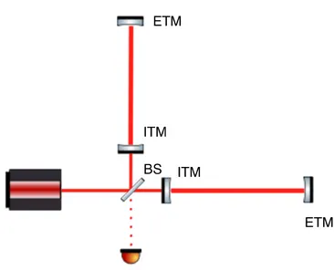
Figure 2.2: A Michelson interferometer with Fabry-Pérot arm cavities. Labeled are theinput test masses (ITMs),end test masses (ETMs), and thebeamsplitter
(BS).
methods of increasing the displacement-to-phase response of the arms. One way to
do this is to install Fabry-Pérot cavities into the arms, as shown in Fig.2.2.
To understand how this works, consider the cavity drawn schematically in Fig.2.3,
and let us compute the fields Erefl and Etrans as a function of the input field Ein = E0eiω0t (i.e., the input-output relation). The field just inside the input mirror is
E1 =itiEin+riE3. (2.12)
But we also know that
E3=ree2ik L
E1, (2.13)
so
E1 =itiEin+riree2ik LE
1. (2.14)
Therefore, recursively,
E1= iti
1−riree2ik L
!
Using this, we can find the intracavitycirculating power:
Pcirc = |E1|2= *
,
t2 i
1+ri2r2e −2rirecos(2k L)
+
-|Ein|2.
(2.16)
In particular, in theresonantcondition where 2k L =n×2π,
G≡ Pcirc
Pin res = ti
1−rire
!2
, (2.17)
wherePin = |Ein|2andGis known as the cavitypower gain.
Figure 2.3: Diagram of a Fabry-Pérot cavity.
We can also now find the transmitted and reflected fields:
Etrans = iteE2=iteeik LE1 (2.18)
= −titeeik L 1−riree2ik L
!
Ein
Erefl = riEin+itiE3=riEin+itiree2ik LE
1 (2.19) =
ri−*
,
t2 iree2
ik L
1−riree2ik L
+ - Ein
= ri−ree2ik L 1−riree2ik L
!
Ein.
Consider the caseri = re ≡ √
R, where Ris the power reflection coefficient, so that
ti =tr ≡√T =
√
1−R. This case, where the input and end mirrors are identical, is
calledcritical coupling. Here, we have
Ptrans Pin =
|Etrans|2
|Ein|2 =
T2
1+R2−2Rcos(2k L) (2.20)
Prefl Pin =
|Erefl|2
|Ein|2 =
2R[1−cos(2k L)] 1+R2−2Rcos(2k L)
17
Therefore, on resonance,
Ptrans Pin res
= T2
(1−R)2 =1 (2.22)
Prefl Pin res
= 0, (2.23)
and the cavity is perfectly transmitting.
Now consider the case when the end mirror is perfectly reflecting (i.e., re = 1)1.
Assuming there are no optical losses in the system, all the power must be reflected
regardless of the resonance condition. Using (2.19), however, we can see that the
phase changes as we sweep the cavity from anti-resonant to resonant:
Erefl=
Ein anti-resonant
−Ein resonant
. (2.24)
Differentiating that equation with respect toLand evaluating on resonance, we find:
dErefl
dL
res
=2ik 1+ri 1−ri
!
Ein. (2.25)
As expected, the derivative is imaginary, meaning the response is in phase.
Com-paring this result with what we would get for a simple reflecting mirror with no input
mirror (i.e.,ri = 0), we see that the phase response is increased by the factor in the parentheses2. That is,
dφrefl
dL
cavity
= 1+ri 1−ri
!
dφrefl
dL
mirror
. (2.26)
Thus, via (2.7), the response of the Michelson to gravitational waves is increased by
this factor when Fabry-Pérot cavities are introduced into the arms.
2.1.1.4 Power recycling
As we’ll see in more detail in below, the SNR of the interferometer with respect to
certain sources of noise originating from the laser is maximized very close to the
dark fringe, where the differential arm phase is∆φ ≈ π. Here, according to (2.7),
Pout ≈ 0 and nearly all the light entering the interferometer is eventually reflected
1
A cavity for whichre >riis calledovercoupled; ifre<ri, it is calledundercoupled, though this case is not often used.
2
back towards the laser3. Given this obvious waste, one can ask how we might reuse
this power leaving the interferometer.
In reality, not all the light entering the interferometer is sent back to the laser, even
on the dark fringe; since all optical systems exhibit some loss (e.g., from scattering
and absorption, etc.), some light is lost in the arms. This loss is enhanced by the
arm cavities: if the power loss over a single roundtrip of the arm cavity isarm, the
light power being constantly lost from the overall system is
Plost= 2armParm =armGarmPin. (2.27)
With this in mind, we can imagine that the entire Fabry-Pérot Michelson
interfer-ometer (FPMI) is just a mirror with amplitude transmission coefficient
tFPMI =parmGarm. (2.28)
Therefore—by analogy with (2.22) and (2.23)—if we place a new mirror between
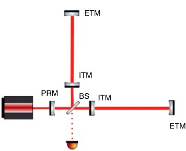
the laser and the BS (as shown in Fig. 2.4) and set its transmission coefficient to
tPRM = tFPMI, we critically couple the light to these integrated losses, maximizing
both the storage time and circulating power within the interferometer. In this
configuration, no wasted light emerges back at the bright port.
To calculate the power recycling enhancement, we need the arm cavity power gain:
Garm≈ tITM 1−rITM
!2
≈ 4
t2 ITM
, (2.29)
where we have used the approximation arm t2ITM 1. Therefore, we choose tPRM= 2
√
arm
tITM , giving4
GPRC = 1 TPRM =
TITM
4arm
, (2.30)
where “PRC” refers to thepower recycling cavity created between the PRM and the average of the two ITMs.
Since the optical power incident on the BS is nowGPRCPin, we have increased the
sensitivity of the instrument to GWs by this PRC gain via (2.7). Note also that the
circulating power in the arms is now
PPRFPMI
arm =
GPRCGarmPin
2 . (2.31)
3Due to this choice of operating point, the symmetric and anti-symmetric ports are also known
as thebright portanddark port, respectively.
4Here and elsewhere we will use the notationT
X≡t2XandRX≡rX2, with upper-case letters
19
Figure 2.4: A Michelson interferometer with Fabry-Pérot arm cavities and power recycling. The added mirror between the laser and the BS is called the power
recycling mirror (PRM).
2.1.1.5 The gain-bandwidth tradeoff
The improvements that come from resonant enhancement of the detector do not
come without a cost. Simply put, the increase in gain is the result of photons
circulating for a longer period of time within the optical system; this increase in
storage timeresults in a corresponding decrease in the detection bandwidth.
To understand this effect, it is useful to introduce the concept of modulation.
Con-sider a laser with input field amplitudeE0and angular frequencyω0passing through
an element that had the ability to apply a phase shift∆φm(t) = Γcos(ωmt). This results in an output field
Eout = E0eiω0t+Γcos(ωmt).
Using the Jacobi-Anger expansion,
eizcosθ = ∞
X
n=−∞
inJn(z)einθ, (2.33)
where Jn(z) is the nth Bessel function of the first kind, this gives the first-order expansion:
Eout ≈ E0eiω0t J
0(Γ)+i J1(Γ)e
iωmt+i J
1(Γ)e −iωmt
(2.34)
≈ E0eiω0t
1+ i
Γ
2 e
iωmt+ iΓ
2e
−iωmt
! ,
where we have used the approximations J0(z) ≈ 1 and J1(z) ≈ z
2 for z 1.
Examining this expression and boosting into the frame of the carrier phasor rotating
in the complex plane at angular frequencyω0, we see that there are three components:
1) a DC field with amplitude E0; 2) a field at relative angular frequency+ωm with amplitude E02Γ; 3) a field at relative angular frequency−ωm, also with an amplitude
E0Γ
2 .
The intuitive time-domain picture of this modulated field is a phasor whose
ampli-tude is not changing, but whose phase is fluctuating—i.e., deviating from a linear
accumulation of ω0t in time—by the sinusoidal factor ∆φm(t). However, this
ex-pansion allows us to treat the phase modulation sidebands (SBs)as independent frequency components of the laser field, and these sidebands can be used to compute
the dynamic response of a system.
For example, one way of modulating the phase of a laser is to reflect it off of a
moving mirror. Indeed, we have already been considering how a
length-change-induced phase shift between two orthogonal arms in a Michelson interferometer
can lead to power modulations (i.e., signal) at its output port, and how installing resonant cavities in those arms can amplify this displacement-to-phase response. In
doing so, we found in (2.26) that this resonant enhancement was proportional to the
arm cavity power gainGarm. However, this was the gain evaluated on resonance.
Since the carrier is resonant, the sidebands are necessarily not on resonance, and this will affect the AC response of the cavity to mirror displacement.
Using (2.16), (2.17) and the relation k = ωc we can define the frequency-dependent
cavity power gain
G(ω)= *
,
t2 i
1+ri2r2e −2rirecos(2
ωL c ) + -= * . . , ti
1−rire 2
1+ (1−r4riirree)2sin2(
ωL c ) + / /
-≡ G(0) 1+F(ω) .
21
It is clear from this expression that the low-frequency gain G(0) is linked to the rapidness of the high-frequency rolloff, embodied by F(ω). We can use F(ω) to find the so-calledhalf-width half-maximum (HWHM)frequency at whichG(ω) is reduced by a factor of two. To do this, we setF(2πfHWHM)= 1, and therefore
fHWHM= c
2πLarcsin
1−rire 2
√
rire
!
. (2.36)
In general, cavities can be built with an arbitrary macroscopic length L. Therefore,
we would like to have a length-invariant measure of the sharpness of a cavity’s
resonance. To get this, we can compare the HWHM frequency to another frequency
scale: thefree spectral range (FSR). This quantity, equal to
νFSR = c
2L, (2.37)
is the spacing in optical frequency between adjacent cavity resonances. Using these
two frequency scales, we can define thefinesse:
F ≡ νFSR 2fHWHM
= π
2 arcsin
1−rire
2√rire
≈
π√rire
1−rire ≈ 2π
tot, (2.38)
wheretot =Ti+Te = (1−ri2)+(1−r2e) 1 is the total roundtrip power loss of
the cavity5. Finally, in the high-finesse limit, the resonant power gain is related to
the finesse by
G(0) =
F
π critically coupled (re =ri)
2F
π fully overcoupled (re= 1).
(2.39)
Now, in (2.26), we saw that the DC length-to-phase response of the arm cavity is
proportional toG(0). Naively then, we might expect the AC response to go asG(ω), but we would be wrong. To see why, imagine that the modulated laser from (2.32)
was injected into the arm cavity before the modulation was applied. The resonant
carrier field amplitude becomes
|E0,cav| =
p
G(0)E0 (2.40)
so the sidebands are generated with seed amplitude
|E(0) ± |=
√
G(0)E0Γ
2 . (2.41)
5At this point, we are only considering the “losses” we intentionally introduce in the form of the
transmissions of the cavity mirrors; in practice, there are always true losses (e.g., from scatter and
Since they are born within the cavity, they are resonantly enhanced by the factor √
G(ωm), giving the output signal SB amplitude6
|E±(ωm)| =
√
G(0)G(ωm)E0Γ
2
∝ G(0) 1+ 2πfωm
HWHM
(forωm 2πνFSR) . (2.42)
Therefore, the DC response of the system to phase or length fluctuations is
propor-tional to the cavity power gain, however, the AC frequency dependence is that of the
amplitude gain. This high-frequency rolloff approximates a single-pole low-pass
filter at frequencies well belowνFSR. For this reason, the HWHM frequency is often
referred to as thecavity polefrequency, fp.
Most saliently, we can see from (2.38) and (2.39) that the product G(0)fp is a constant for a given fixed cavity length—this is the essence of the gain-bandwidth
tradeoff.
2.1.1.6 Coupled cavities
Treating the PRC as a cavity with the PRM as an input mirror and the FPMI as an
effective end mirror is not the only way to view the system. From the perspective
of a photon circulating in the arm cavity, for example, things look wholly different.
To such a photon, the effect of the PRM depends very much on whether there is a
complementary photon in the other arm cavity: since the Michelson is being held
on the dark fringe, common-modesignals generated in the two arms will interfere constructively when they reach the BS and be sent towards the symmetric port,
whiledifferential-modesignals will interfere destructively and be sent towards the anti-symmetric port.
In other words, photons corresponding to common signals between the two arms
(e.g., signals originating from the laser in the first place, or signals caused by
common-mode displacements of the arm cavity lengths) will see the influence of
the PRM, while differential-mode signals (e.g., changes in the length of only one
of the arm cavities, or—as we’ll see later—optical field fluctuations entering the
interferometer from the anti-symmetric port), have no way of knowing it’s there;
on the other side of the ITM, a differential-mode signal simply sees the dark port.
Therefore, to understand this coupled cavitysystem, we must consider these two types of signals separately.
6By analogy with (2.15), the resonant sideband field enhancement is actually
√
G(ωm)
i ti , but this
intracavity field must be multiplied by the input mirror field transmissionitito get the signal sideband
23
In the case of the common-mode signals, due to the gain-bandwidth relationship
discussed in the previous section (i.e., since fp∝ G1), we can calculate thecoupled
cavity pole:
fp,cc = fp
2GPRC
. (2.43)
That is, the increase in DC gain by the factor GPRC comes with a reduction in
bandwidth by the same factor7. In this case, there isn’t much of a tradeoff: since
the signal enhancements we have been calculating come from the amplification of
the DC power, P0, we don’t really care that the bandwidth of this coupled cavity
has been reduced; as we’ll see in a moment, the differential-mode signal SBs are
unchanged by this effect.
In fact, the narrowing of this cavity is actually beneficial in many ways. For example,
consider the effect of input laser power fluctuations. Rewriting the input power as
P0→ P(t)= P0+δP(t), (2.44)
we can examine the effect of δP(t) on the measured interferometer signal at the
AS port. First, consider the simple Michelson case. Using (2.7) and recalling that
we are operating at a small offset δφfrom the dark fringe (i.e.,∆φ= π+δφ, with
δφ π), we have
PMI
out(t)≈ (P0+δP(t))
δφ2
4 (2.45)
Therefore, the power fluctuation δP(t) is passed directly to the output port by
the factor δφ2/4. Comparing this to the effect of a true signal (e.g., by writing
∆φ(t) = π+δφ+2k Lh(t)), we measure
PMI
out(t)≈ P0
δφ2
4 +
δφ2
4 δP(t)+2k LP0δφh(t). (2.46)
Analyzing the fluctuating terms, we see that the power noise couples to the apparent signal as8
hMI app.(t) =
δφ
8k L
δP(t)
P0 . (2.47)
7
The factor of two comes from the fact that the ratio ofGtoF changes by a factor of two when
going from a fully overcoupled cavity to a critically coupled cavity.
8
This result shows two important features of laser intensity noise: 1) the coupling is smaller as
we approach the dark fringe, and 2) the important quantity is not the absolute noiseδP(t), but rather
Now, let’s consider what happens when we introduce power recycling and arm
cavities. In this case, switching to frequency space, (2.46) becomes9,10
PPRFPMI
out (f) ≈GPRCP0
δφ2 4 + * . , GPRC
1+ fpi f,cc
+ /
-δφ2
4 δ
P(f)+* .
,
GPRCGarm
1+ i ffp
+ /
-2k LP0δφh(f),
(2.48)
where here and for most of the rest of this thesis we will use the natural Fourier
frequency, f = 2ωπ. Comparing (2.46), (2.48) and (2.47), we discover:
hPRFPMI app. (f)
hMI app.(f)
= 1
Garm
* .
,
1+ i ffp
1+ fpi f,cc
+ /
-. (2.49)
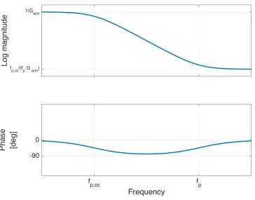
Apart from the expected factor of Garm due to the arm cavities, we also see an
improvement in the region fp,cc < f < fp, where the coupling of laser power
fluctuations to the output has started falling off due to the coupled cavity pole, but
the interferometer’s response to GWs has not started falling off due to the arm cavity
pole. In this case, then, the reduction of the coupled cavity bandwidth has helped
us. This improvement in laser power noise coupling is plotted in Fig.2.5.
2.1.1.7 Signal recycling/extraction
Using the common/differential-mode selectivity of the Michelson on its dark fringe
to create two decoupled optical systems begs the question: by extension of the
power recycling concept, can we apply the same technique to the differential mode
by adding a new mirror a the dark port, as shown in Fig.2.7? The answer is “yes.”
To understand what is possible with this extra signal recycling mirror (SRM), it is helpful to consider the power recycling case from a different angle. In the
previ-ous section, we determined fp,cc heuristically by appealing to the gain-bandwidth
relation. However, we can arrive at the coupled cavity dynamics more directly by
looking at it as a cavity made of the ETM on one side, and a compound mirror
formed by the ITM and the PRM on the other side, as shown in Fig.2.6.11
9
While it is a power quantity, the middle term here proportional toδP(f)is still modified by the
amplitudefactor in the parentheses. This is becauseδP(t)comes from a cross term between the DC carrier field and a fluctuating amplitude modulation SB. Only the latter part of the product carries frequency dependence, while both carry the DC amplitude gain of
√
GPRC.
10
The phase information here is inserted by analogy with that required by the Kramers-Kronig relations for the minimum-phase single-pole low-pass filter that the cavities approximate in the low-frequency limit.
11
25
[image:40.612.110.474.114.399.2]Figure 2.5: Transfer function from input laser power noise to apparent GW signal in a PRFPMI, normalized by that for a simple Michelson.
Using (2.18), we can calculate the power transmission of the PRC as
TPRC(ω) =t2
PRC(ω) =
TPRMTITM
1+RPRMRITM−2
√
RPRMRITMcos(2ωLPRC
c )
. (2.50)
When the PRC is anti-resonant, this becomes
TPRC anti−res
≈ TPRMTITM
4 . (2.51)
Now, in this picture, the coupled cavity uses the anti-resonant PRC as compound
mirror designed to critically couple the input light to the arm lossesarm. Therefore,
we expect the finesse to be
Fcc = 2π
TPRC+arm =
2π
2TPRC
≈ 4π
TPRMTITM, (2.52)
and, since this is a critically coupled cavity, the power gain is
Gcc = Fcc
π ≈
4
TPRMTITM. (2.53)
If the two pictures are consistent, this should be equal toGPRCGarm. Using (2.29)
and (2.30), we indeed find:
GPRCGarm= 1 TPRM
4
TITM =Gcc. (2.54)
As for the coupled cavity pole, we can compute the expected value as
fp,cc =
Farm Fcc fp=
2π
TITM
TPRMTITM
4π =
TPRM
2
fp= fp
2GPRC
, (2.55)
which is what we found in (2.43).
From this new perspective, we can see how adding an SRM will affect the differential
mode. For example, if we chooseTSRM =TPRMand the same anti-resonant condition
for the SRC, then the differential-mode signal sidebands will experience the same
augmentation as the carrier field and the common-mode fluctuation SBs. Namely,
they will be enhanced at low frequencies by the extra factor √
GPRC, but they will
also be band-limited by the same coupled cavity pole fp,cc = fp
2GPRC. This application
is the eponymous signal recycling, and it has been used in the non-Fabry-Pérot-enhanced GW interferometer GEO600 [21]12.
On the other hand, if we make the SRCresonant, this makes it highly transmissive from the dark port into the arms. In this case, the differential coupled cavity is
12Due to GEO600’s relatively short arms and lack of arm cavities, true signal recycling results in
27
Figure 2.7: The full core aLIGO optical configuration: a dual-recycled Fabry-Pérot Michelson interferometer (DRFPMI). The lengths Lx,Ly,lx,ly,l0p and l0s will be
used to define the interferometer’s length DoFs in Sec.2.1.2.4.
strongly overcoupled with very low finesse. Therefore, the low-frequency gain will
be reduced by the factor √
GSRC—less than one due to the anti-resonant state—and
the bandwidth will be increased in proportion to G1
SRC. Since, in this case, the SRC
would be a relatively high-finesse cavity, the reduction in gain would be too great,
even in light of the increased signal bandwidth. However, by choosing TSRM TPRM, we can use this effect to a reasonable degree, increasing the differential
coupled cavity pole frequency (with respect to the naked arm) by
fp,cd fp =
1
GSRC (2.56)
while only reducing the signal gain by the factor √
GSRC. This application is called
resonant sideband extraction (RSE)[29], and it is how the SRM is primarily used
in aLIGO. A significant advantage to this scheme is that it allows one to increase the
sensitivity—without sacrificing bandwidth. This alleviates the thermal heating of
the BS and ITM substrates, which can lead to optical aberrations.
Finally, the SRC can also be operated in a phase condition which is neither resonant
nor anti-resonant. This configuration, called detuned signal recycling, has two main consequences. First, due to the displacement of the cavity resonance from the
carrier frequency, the interferometer will have a heightened response to
differential-mode signals of a frequency equal to this detuning (since either the upper or lower
sideband will coincide with the coupled cavity resonance). This results in an
interferometer response that is peaked at the detuning frequency, but diminished
everywhere else with respect to the tuned RSE case. This allows for tuning the
interferometer to sources of a specific, narrow spectral range


![Figure 2.8: More accurate diagram of the aLIGO optical layout. (Image source:[23])](https://thumb-us.123doks.com/thumbv2/123dok_us/315350.1032605/45.612.110.509.66.366/figure-accurate-diagram-aligo-optical-layout-image-source.webp)
![Figure 2.10: Advanced LIGO PSL. (Image source: [23])](https://thumb-us.123doks.com/thumbv2/123dok_us/315350.1032605/48.612.111.511.76.276/figure-advanced-ligo-psl-image-source.webp)