2017 International Conference on Mathematics, Modelling and Simulation Technologies and Applications (MMSTA 2017) ISBN: 978-1-60595-530-8
A Set of Ternary Time Series Forecasting Models
Based on the Difference Rate
Xiao-li LU, Hong-xu WANG, Cheng-guo YIN, Hao FENG and Qing-yan WU
Hainan Tropical Ocean University, Sanya, Hainan, China, 572022
Keywords: Difference rate, Set of ternary time series forecasting models, The prediction function of ASTDR.
Abstract. A set of ternary time series forecasting models based on the difference rate (ASTDR) is proposed. For an arbitrary time series, we can apply automatic optimization search method to sieve the ordinary time series forecasting model in ASTDR. For example, when simulating the prediction of the enrollments of University of Alabama in 1971–1992, we can apply automatic optimization search method to sieve the ordinary time series forecasting model Ft(0.000003,0.7, 0.000003) in ASTDR. The mean square error (MSE) and the average forecasting error rate (AFER) of the predicted values of the enrollments can reach MSE=0 and AFER=0%. The prediction accuracy of simulating the prediction of historical data of time series reaches the most ideal level.
Introduction
This paper is a generalization of the forecasting model proposed by Wang and Wu [1] and Feng, Wang, Yin, and Lu [2], in which [1] focuses on the theoretical study of forecasting method, and [2] focuses on: when the enrollments of University of Alabama in 1971–1992 are simulated and predicted, the method is compared with the existing fuzzy time series forecasting models. These two papers are all aimed at the case that the prediction function is a binary function. This paper further promotes them to the case that the prediction function is ternary function. A set of ternary time series forecasting models based on the difference rate (ASTDR) is proposed. The concept of the ordinary time series forecasting model is proposed. When the forecasting model is used to simulate the historical data of a certain time series, the mean square error of the predicted value is MSE=0, and the average forecasting error rate is AFER=0%. For any time series, we can use the automatic optimization search method to sieve the ordinary time series forecasting model in ASTDR. Example 1. When simulating the prediction of the enrollments of University of Alabama in 1971–1992, we can apply automatic optimization search method to sieve the ordinary time series forecasting model Ft(0.000003,0.7,0.000003) in ASTDR. The prediction accuracy of simulating the prediction of historical data of time series reaches the most ideal level. The forecasting model of this paper has obvious advantages over the existing fuzzy time series forecasting models (such as [5–16]).
A Set of Time Series Forecasting Models Represented by Astdr
Definition 1. Let U = {U1, U2, …, Un} be the universe of discourse of historical data of a time series. The calculation formula of year by year difference rate of historical data is St = (Ut – Ut-1) /Ut-1, and the universe of discourse S = {S2, S3, ..., Sn} of the difference rate of historical data is obtained.
Definition 2. Let U = {U1, U2, …, Un} be the universe of discourse of historical data of a time series. Let S = {S2, S3, ..., Sn} be the universe of discourse of year by year difference rate of historical data. Define on S:F g h kt( , , )Ut1
1V g h kt( , , )
It is the prediction function of ASTDR, where the independent variables g(0,1), h(0,1),
2 3
1
, 2,
( , , )
, {3, 4, , }.
t t t h k t h k S S
V g h k
g h
t n
g h
S S
If the independent variables g, h, and k choose the specific values in their respective universe of discourse, a prediction formula Ft(g, h, k) can be established. For a time series, the prediction formula Ft(g, h, k) can simulate the prediction of the historical data of the time series, so Ft(g, h, k) is a time series forecasting model.
Definition 3. Let U = {U1, U2, …, Un} be the universe of discourse of historical data of a time series. Let S = {S2, S3, ..., Sn} be the universe of discourse of year by year difference rate of historical data. When the independent variables g, h, k take all the specific values in their respective universe of discourse, infinite time series forecasting models Ft(g, h, k) can be obtained. The whole of all the time series forecasting models Ft(g, h, k) is called a set of ternary time series forecasting models based on the difference rate (ASTTSFMBDR), further simplify the abbreviation as ASTDR. The general element of ASTDR is Ft(g, h, k). Ft(g, h, k) represents the prediction formula of a time series forecasting model, it also represents a time series forecasting model using Ft(g, h, k) as prediction formula.
Definition 4. If the forecasting model is used to simulate the prediction of the historical data of the time series, the MSE of the predicted values is MSE=0, and AFER=0%, then the time series forecasting model Ft(g, h, k) is called ordinary.
Definition 5. For a time series, the standard time series forecasting model in ASTDR is automatically searched by computer, this method is called automatic optimization search method. The concrete steps are: for a time series, from a group of decimal g(0,1), h(0,1), k(0,1) as the starting point of programming, programming, searching, and computing, ..., until the ordinary time series forecasting model Ft(g, h, k) in ASTDR is sieved (satisfying AFER=0%, MSE=0).
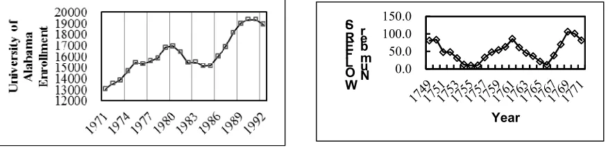
Example 1. The enrollments of University of Alabama in 1971–1992 given by Song and Chissom [3] are shown in TABLE II, their distribution diagram is shown in FIGURE I. FIGURE I shows that the enrollments of University of Alabama in 1971–1992 are a time series, which are irregular time series.
In simulating the prediction of the enrollments of the University of Alabama in 1971–1992, from h=0.7, g=k=0.0003 as the starting point of programming, select h=0.7, g=k=0.0003; h=0.7, g=k=0.00003; h=0.7, g=k=0.000003; ..., by programming, searching, computing, ..., until the ordinary time series forecasting model Ft(g, h, k) in ASTDR is selected (AFER=0%, MSE=0). Firstly get TABLE 1, for AFER=0.0085%≠0% and MSE=16.6667≠0; continue searching and calculating, then get TABLE2, for AFER=0.0008%≠0% and MSE=0.2381≠0; continue searching and calculating, finally get TABLE 3,
[image:2.612.91.529.555.663.2]0.0 50.0 100.0 150.0 W O L F E R 'S N u m b e r Year
Figure 1. Distribution diagram of the enrollments of University of Alabama in 1971–1992.
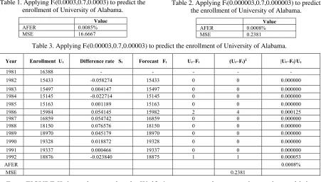
Figure 2. Distribution diagram of wolfer’s sunspot numbers in 1749–1771.
Table 1. Applying Ft(0.0003,0.7,0.0003) to predict the
enrollment of University of Alabama.
Value
AFER 0.0085% MSE 16.6667
Table 2. Applying Ft(0.000003,0.7,0.000003) to predict
the enrollment of University of Alabama.
Value
AFER 0.0008% MSE 0.2381
Table 3. Applying Ft(0.00003,0.7,0.00003) to predict the enrollment of University of Alabama.
Year Enrollment Ut Difference rate St Forecast Ft Ut–Ft (Ut–Ft)2 |Ut–Ft|/Ut
1981 16388 - - - - -
1982 15433 -0.058274 15433 0 0 0.000000
1983 15497 0.004147 15497 0 0 0.000000
1984 15145 -0.022714 15145 0 0 0.000000
1985 15163 0.001189 15163 0 0 0.000000
1986 15984 0.054145 15982 2 4 0.000125
1987 16859 0.054742 16859 0 0 0.000000
1988 18150 0.076576 18150 0 0 0.000000
1989 18970 0.045179 18970 0 0 0.000000
1990 19328 0.018872 19328 0 0 0.000000
1991 19337 0.000466 19337 0 0 0.000000
1992 18876 -0.023840 18875 1 1 0.000053
AFER 0.0008%
MSE 0.2381
From FIGURE II, it can be seen that the Wolfer’s sunspot numbers are a time series, and it is an irregular time series.
In simulating the prediction of Wolfer’s sunspot numbers in 1749–1771, from h=0.5, g=k=0.0001 as the starting point, select h=0.5, g=k=0.0001; h=0.5, g=k=0.00001; h=0.5, g=k=0.000001; ..., by programming, searching, computing, ..., until the standard time series forecasting model Ft(g, h, k) in ASTDR is selected (AFER=0%, MSE=0). Firstly get TABLE IV, for AFER=0.1195%≠0% and MSE=0.017≠0; continue searching and calculating, then get TABLE V, for AFER=0.0261%≠0% and MSE=0. 0009≠0; continue searching and calculating, finally get TABLE VI, because AFER=0%, MSE=0, stop the calculation. Therefore, Ft(0.000001,0.5,0.000001) is ordinary time
series forecasting model in ASTDR when simulating the prediction of Wolfer’s sunspot numbers in 1749–1771.
[image:3.612.78.534.544.747.2]Example 2. Yule [4] studied the time series—Wolfer’s sunspot numbers for the first time in 1927. Because the number of samples is large, for convenience, we only take a part of them, namely take Wolfer’s sunspot numbers in 1749–1771 to study. The specific data are shown in TABLE4, and its distribution diagram is shown in FIGURE II.
Table 4. Applying Ft(0.0001,0.5,0.0001) to Predict Sunspot Numbers.
Year WOLFER’S number
Ut
Difference rate St Forecast Ft (Ut-Ft)2 |Ut-Ft|/Ut
1760 62.9 -- --- --- ---
1761 85.9 0.365660 85.9 0.000000 0.000000 1762 61.2 -0.288126 61.1 0.000000 0.000000 1763 45.1 -0.262469 45.1 0.000000 0.000000 1764 36.4 -0.194013 36.3 0.010000 0.002751 1765 20.9 -0.425034 20.9 0.000000 0.000000 1766 11.4 -0.454545 11.4 0.000000 0.000000 1767 37.8 2.315789 37.8 0.000000 0.000000 1768 69.8 0.846561 69.8 0.000000 0.000000 1769 106.1 0.520057 106.1 0.000000 0.000000 1770 100.8 -0.049953 100.8 0.000000 0.000000 1771 81.6 -0.190476 81.6 0.000000 0.000000
AFER 0.1195%
Table 5. Applying Ft(0.00001,0.5,0.00001) to Predict
Sunspot Number. Table 6. Applying FPredict Sunspot Numbers. t(0.000001,0.5,0.000001) to
Value Value
AFER 0.0261% AFER 0.0000%
MSE 0.0009 MSE 0.0000
Conclusions
For a time series, the ordinary time series forecasting model in ASTDR can be automatically searched and sieved by using computer, and make MSE=0 and AFER=0%. TABLE III shows that Ft(0.000003,0.7,0.000003) is an ordinary time series forecasting model in ASTDR when simulating the prediction of the enrollments of University of Alabama in 1971–1992; TABLE VI shows that Ft(0.000001,0.5,0.000001) is an ordinary time series forecasting model in ASTDR when simulating the prediction of Wolfer’s sunspot numbers in 1749–1771. The prediction accuracy of simulating the prediction of the historical data of the time series has reached the most ideal level.
Acknowledgment
This work is supported by Natural Science Foundation of Hainan Province (Grant No.714283), and QYXB201301, 2016YD04,2015YD33.
References
[1] Wang Hongxu and Wu Zhenxing, “Preliminary Theory of Set SDR of Fuzzy Time Series Forecasting Model,” 2016 International Conference on Mathematical, Computational and Statistical Sciences and Engineering (MCSSE2016). pp. 261–265, 2016.
[2] Hao Feng, Hongxu Wang, Chengguo Yin, and Xiaoli Lu, “The Set SFmBDR of Fuzzy Time Series Forecasting Models,” 2017 2nd International Conference on Modelling, Simulation and Applied Mathematics (MSAM2017). pp. 45–48, 2017.
[3] Q. Song and B.S. Chissom, “Forecasting enrollments with fuzzy time series—Part I,” Fuzzy Sets and Systems. vol. 54, pp. 1–9, 1993.
[4] G. Udny Yule, “On a Method of Investigating Periodicities in Disturbed Series, with Special Reference to Wolfer's Sunspot Numbers,” Philosophical Transactions of the Royal Society. A: Mathematical, Physical and Engineering Sciences, vol. 226, pp. 267–298, 1927.
[5] R.C. Tsaur, J.C.O. Yang, and H.F. Wang, “Fuzzy relation analysis in fuzzy time series model,” Comput. Math. Appl. vol. 49, pp. 539–548, 2005.
[6] C.H. Cheng, T.L. Chen, H.J. Teoh, and C.H. Chiang, “Fuzzy time series based on adaptive expectation model for TAIEX forecasting ,” (MEPA), Expert Syst. Appl. vol. 34, pp. 1126–1132, 2008.
[7] V.R. Uslu, E. Bas, U. Yolcu, and E. Egrioglu, “A fuzzy time series approach based on weights determined by the number of recurrences of fuzzy relations,” Swarm and Evolutionary Computation. vol. 15, pp. 19–26, 2014.
[8] Bhagawati P. Joshi and Sanjay Kumar, “A computational method for fuzzy time series forecasting based on difference parameters,” International Journal of Modeling, Simulation, and Scientific Computing. vol. 4, No. 1, pp. 1250023–1–1250023–12, 2013.
[10]H.X. Wang, J.C. Guo, H. Feng, and Hailong Jin, “An improved forecasting model of fuzzy time series,” Advances in Mechatronics and Control Engineering Ⅲ. Edited by Prasad Yarlagadda, Applied Mechanice and Materials. vol. 678, pp. 64–69, 2014.
[11]H.X. Wang, J.C. Guo, H. Feng, and F.J. Zhang, “A new model of forecast enrollment using fuzzy time series,” IRAICS proceedings series 7, Education Management and Management Science, International Research Association of Information and Computer Science. VOLUME 7, 2014 International Conference on Education Management and Management Science (ICEMMS 2014), 7– 8 August. pp. 95–98, 2014.