How does duration between trades of underlying securities affect option prices?

BIROn - Birkbeck Institutional Research Online

Cartea, Alvaro and Meyer-Brandis, T. (2007) How does duration between

trades of underlying securities affect option prices? Working Paper. Birkbeck,

University of London, London, UK.

Downloaded from:

Usage Guidelines:

Please refer to usage guidelines at or alternatively

ISSN 1745-8587

Birkbeck Workin

g

Pa

p

ers in Economics & Finance

School of Economics, Mathematics and Statistics

BWPEF 0721

How Does Duration between Trades

of Underlying Securities Affect

Option Prices

Alvaro Cartea

Birkbeck, University of London

Thilo Meyer-Brandis

CMA, University of Oslo

How Does Duration Between Trades of Underlying

Securities Affect Option Prices

∗

´

Alvaro Cartea

Birkbeck, University of London, UK

Email: [email protected]

Thilo Meyer-Brandis

CMA, University of Oslo

Email: [email protected]

November 26, 2007

∗_{First Version April 2004. Corresponding author [email protected]. This paper has benefited from}

com-ments of seminar participants at The University of Chicago, Federal Reserve Bank Chicago, University of Flo-rence, University of Toronto, University of Oxford, ESSEC, King’s College London and Birkbeck-University of London. For comments and suggestions on earlier drafts, we are indebted to Gene Amromin, Luca Benzoni, Raymond Brummelhuis, Marcelo G. Figueroa, Craig Furfine, Helyette Geman, Sam Howison, Aytac Ihlan, Se-bastian Jaimungal, Tim Jenkinson, Pete Kyle, David Marshall, Dilip Madan, Colin Mayer, Robert McDonald, Roel Oomen, Andrea Roncoroni, Oren Sussman and Jos van Bommel.

†_{A. Cartea is thankful for the hospitality and generosity shown by the Finance Group at the Sa¨ıd Business´}

ABSTRACT

We propose a model for stock price dynamics that explicitly incorporates random

waiting times between trades, also known as duration, and show how option prices can be

calculated using this model. We use ultra-high-frequency data for blue-chip companies

to motivate a particular choice of waiting-time distribution and then calibrate risk-neutral

parameters from options data. We also show that the convexity commonly observed in

implied volatilities may be explained by the presence of duration between trades.

Further-more, we find that, ceteris paribus, implied volatility decreases in the presence of longer

durations, a result consistent with the findings of Engle (2000) and Dufour and Engle

(2000) which demonstrates the relationship between levels of activity and volatility for

stock prices.

Keywords: Duration between trades, waiting-times, high frequency data, L´evy processes,

Most financial models assume that securities are continuously traded. However, in equity markets for example, trading happens discretely at random times. In the literature there have been several approaches to directly model the times between trades also known as duration. Early models that capture the impact of duration between trades include Diamond and Ver-rechia (1987) and Easley and O’Hara (1992). The work of Easley and O’Hara establishes the link between the existence of information, the timing of trades and the dynamics of security prices. One of their main contributions is to show that duration between trades affects the behavior of security prices and consequently that transaction prices are not a Markov process, as is currently assumed in many financial models.

Using ultra-high-frequency equity data, Engle (2000) studies the consequences of stochas-tic trade arrival times (see also Engle and Russell (1998)). This empirical study finds evidence that both stock returns and variances are found to be negatively influenced by long durations between trades. The study of Dufour and Engle (2000) shows that the stochastic component of duration can explain the relationship between short time durations, i.e. high trading activity, and both larger quote revisions and stronger positive autocorrelations of trades.

Recent work by A¨ıt-Sahalia and Mykland (2003) focuses on the estimation of continuous-time models and its consequences, in particular the fact that high-frequency financial data are discretely sampled in time and that the time separating successive observations is often random. One of the main messages emerging from their findings is that for empirical purposes, researchers using randomly spaced data, “... should pay as much attention, if not more, to sampling randomness as they do to sampling discreteness”.

When it comes to derivative pricing, most financial literature on discrete time models as-sumes that the distribution of the waiting-timeτn=Tn−Tn−1 between the nth and(n−1)th

trades, occurring at times Tnand Tn−1respectively, is either constant (tree models) or

The first question is not a new line of research in the literature, but the second, despite its importance in asset pricing, has not been addressed until now.

When looking at data that involves the random arrival of events, trades in our case, it is customary to look at what is known as the survival function, which represents the probability that the waiting-time between two consecutive trades is greater than t. This function is given by

ϒ(t) =1₋

Z t

0 υ(

u)du, (1)

whereυ(t)denotes the probability density function (pdf) of the waiting times.

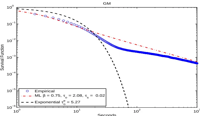
If we assume that the waiting-time between trades possesses an exponential distribution with parameterλ, thenυ(t) =λe−λt andϒ(t) =e−λt. Employing General Motors (GM) con-solidated trades (over the period April-June 2005) in Figure 1, as an example we show a log-log plot of empirical and fitted exponential survival functions.1 We used 419,264 trades from all exchanges with a resulting average duration between consecutive trades ofτe_o=5.26 seconds. The Figure also shows that the fitted exponential survival function with parameter λ=1/τe

o, (the dashed line), is a very poor fit when compared to empirical data (circles).2

100 101 102 103

10−6 10−5 10−4 10−3 10−2 10−1 100

GM All trades, all exchanges

Seconds

Survival Function

Empirical Exponential τe

o = 5.27

Intuitively, the rationale for rejecting the exponential survival function as a possible can-didate to model durations is its inability to capture the long durations between consecu-tive trades, see for example Engle (2000), Engle and Russell (1998) and Dufour and Engle (2000). Furthermore, assuming that the duration between consecutive trades is exponentially distributed is equivalent to assuming that the number of trades follows a Poisson counting pro-cess. If this were the case, then the mean and variance of the data should be the same, a prop-erty know as ‘equidispersion’. In fact, what is commonly observed in ultra-high-frequency models is ‘overdisperion’, i.e. where the variance is greater than the mean of the data, see Cameron and Trivedi (1996). For example, in the case of GM the variance of waiting times for trades is 3.4575_∗103, while the mean is 5.27.

In this article, we concentrate on the question of how derivatives prices are calculated when durations possess a distribution function that better reflects the observed empirical be-havior. Our contribution is threefold. Firstly, we propose a general model that explicitly incorporates waiting times as one of the building blocks of stock price dynamics under the physical measure. Secondly, we show how option prices are calculated by choosing a risk-adjusted measure. Thirdly, based on empirical waiting-time data from blue-chip companies, we investigate a particular distribution for duration and we employ it to calibrate risk-neutral parameters to IBM options data.

Under the risk-adjusted measure we propose the use of a survival function that can capture long waits between trades and that nests, as a particular case, the exponential survival function. We then calibrate our model to IBM options data and find that in the vast majority of the cases the risk-neutral parameters of the stock dynamics responsible for modeling the duration between trades, indicate that the risk-neutral distribution of waiting times is not exponential.

waiting-times that are not exponentially distributed contribute to the implied volatility ob-served in financial markets. In particular, when we assume that price revisions are Gaussian, which asymptotically behaves like the classical Black-Scholes framework, the inclusion of non-exponential waiting-times is solely responsible for the emergence of the convexity in the volatility ‘smile’. We also observe that, ceteris paribus, implied volatility decreases when waiting times are ‘longer’, a finding in line with those of Engle (2000) and Dufour and Engle (2000) which links the relationship of levels of activity and volatility for stock prices.

The rest of this article is organized as follows. Section I proposes a general model for stock prices, under the statistical measure, where duration between trades is random. Section II focuses on the pricing of instruments such as European-style options. Section III justifies the selection of particular waiting-time distributions and shows how European-style option prices may be calculated by employing widespread techniques such as those in Carr and Madan (1999). Section IV calibrates risk-neutral parameters for one of our models, using IBM options data. Section V produces numerical examples of how duration affects the shape and level of implied volatility. Section VI concludes.

I. The Model: spot dynamics with duration

Before presenting the model we need two more definitions: a counting process; and the hazard function. We denote the time of the nth trade by Tnand the duration between trades by Tn−Tn−1=τnwith continuous pdfυ(t). Hence we can write

Tn=T0+

n

∑

τi, Tn−Tn−1=τn, n=1,2,3,···.

The counting process, which represents the number of trades over the interval[0,t], is defined by

Nt=max{n≥0|Tn≤t}.

Further, the hazard function u(t)is defined as

u(t) =₋d

dtlnϒ(t), t∈R

+_{, (2)}

where the survival function ϒ(t) is that given above in equation (1). Intuitively, the hazard function represents the probability that a trade will happen in the next small time interval divided by the length of that time interval; i.e. the hazard function is the instantaneous intensity of a trade occurrence. Here we assume that u(t)is strictly positive and continuous.

Stock price revisions

To model the stock price revisions, we assume that every time there is a trade, i.e. the counting process Nt increases by one unit, the price revision of the logarithm of the stock price X(t) =

ln S(t)moves by i.i.d. Y . More precisely, we assume that the dynamics of the observed tick-by-tick microstructure of X(t), under the physical measureP, are described by

X(t) =X(0) + (r₋D)t+

Nt

∑

where the constants r and D denote the risk-free rate and the dividend yield. Note that for technical convenience, we consider a continuously compounded risk-free behavior with rate

(r₋D) instead of capturing this deterministic trend in the jump price revisions ∑Nt

i=1Yi. At

jump times (i.e. when there is a trade) there is no price difference between these two al-ternatives. However, with the continuous rate technicalities are simplified when it comes to derivatives pricing in section II below. We assume that the i.i.d. spacial shocks Y , which are independent of the waiting times, possess an infinitely divisible distribution. Given the above, the log-characteristic function of Y is given by the L´evy-Khintchine representation

lnEheiξYii_≡Ψ₍ξ_{) =ai}ξ₋1

2σ

2_ξ2₊Z

R\{0}

eiξl₋1₋iξl1_|l|<1W(dl). (4)

Here a_∈R,σ_≥0, the truncation function l1_|l|<1ensures integrability around the origin, and

Ψ(ξ) is known as the characteristic exponent of the distribution with triplet(a,σ2_{,W). For}

technical simplicity, we assume that the distribution of the spacial shocks Y is given by a continuous density g(y)>0, y _∈R. Note that if we denote by N(ω,dt,dz) =N(dt,dz) the integer valued jump measure associated with the process∑Nt

i=1Yi, we can rewrite the dynamics

(3) as3

X(t) =X(0) + (r₋D)t+ Z t

0 Z

R0

z N(dt,dz). (5)

In the financial literature, the two most common models of the type described in equation (3) are: discrete time models (tree models) with deterministic, equally spaced, time stepsτn;

and compound Poisson models where theτn’s are i.i.d. exponentially distributed, random

vari-ables. In the latter, X(t)belongs to the class of L´evy processes which have been extensively studied and applied in finance over the recent years.

For example, a conditionally Gaussian model arises when it is assumed that price revisions in (3) arise from a Gaussian distribution, with Y _∼N(µ,σ2_{), and that the counting process N}

t

price revisions is not supported by empirical studies, especially over short-time periods. Most efforts to improve these models have focused on the spacial shocks aspect, as opposed to the distribution of the waiting timesτ, despite the crucial role that these waiting times play in the distributional properties of stock prices.

A major reason why people only reluctantly depart from exponentially distributed waiting times, is the loss of Markovianity (even if empirical studies confirm the non-Markovianity of prices). Indeed Markovianity is important for many issues, including derivatives pricing, where expectations conditioned on past market evolution have to be computed. With the exception of the exponential waiting-time distribution, the log-stock X(t)is not Markovian for a general waiting-time distribution in model (3). Indeed, let H(ω,t) =H(t) denote the so-called backward recurrence time (i.e. the time elapsed since the last trade) defined by

H(t) =t₋TNt, (6)

where TNt represents the last trade time before t. Then it is well known (see e.g. Jacobsen

(2006)) that the intensity of the counting process Nt is given by u(H(t))Consequently, the

predictable compensator of the jump measure N(dt,dz)is the random measure

ν(ω,dt,dz) =ν(dt,dz):=u(H(t))g(z)dtdz, (7)

where u(t)was the hazard function given in (2) and g(z)the probability density of the shocks

Y . From this it follows that the process is not Markovian as long as u(t) is not constant. Intuitively, for general hazard functions u(t), it is important to know the time elapsed since the last trade and thus the process is not memoryless. However, if we enlarge the state space with the backward recurrence time H(t), then we have the following result.

Theorem 1 The two dimensional process(X(t),H(t)) is a time-homogeneous Markov

This is an important property which we will use below to price options. For a proof see appendix A.

A special example is the well-known case resulting from the assumption that the waiting timesτ are exponentially distributed with parameter λ. For this particular case, the survival function is given byϒ(t) =e−λtand the hazard function becomes u(t) =λ; note that the hazard function is independent of the backward recurrence time H(t). In this case the compensating measure (7) becomes ν2(ω,dt,dz) =λg(z)dtdz, which is the compensating measure of the

compound Poisson process X(t), and it is not necessary to consider the two-dimensional pro-cess(X(t),H(t))because X(t)already is Markovian.

II. Derivatives Pricing

One of the key requirements we have imposed on our model for stock price dynamics is that we can price financial instruments, such as European-style options written on the underlying stock

S(t). Therefore, in the first part of this section, we discuss the possible risk-neutral dynamics exhibited by S(t)when we assume that, under the physical measureP, the stock price follows (3). In the second part we then proceed to discuss derivatives pricing and derive an integro-pde characterization for the price process of European-style options in our framework. Further, under the assumption that a trade just has happened, we derive a second price description based on Fourier transform techniques which is much more efficient in practice both to price, and more importantly, to calibrate risk-neutral parameters.

On our stochastic basis(Ω,

F

F

note that the same filtration is generated by the two-dimensional process(X(t),H(t)). Since

To specify the family of potential EMMs, we adopt the same approach employed by the vast majority of incomplete market models. We assume that the stock dynamics under the risk-adjusted measure have the same structure as under the physical measure. For example, in the L´evy process literature it is assumed that stock prices will follow a L´evy process under both the physical and risk-neutral measure, but not necessarily the same one (Cont and Tankov (2004)).4 Therefore, we will assume that the risk-neutral process will possess the same struc-ture under both measures. In particular, the number of trades will be independent from price revisions, but we allow the distribution of the number of trades to be different under the risk-neutral measure. In addition the distribution of price revisions is again infinitely divisible, but not necessarily the same one as under the physical measure.

More precisely, we assume that the market chooses from a class of EMMs whose densities with respect toPis given by the following stochastic exponentials

dQ

dP =exp

Z t

0 Z

R0

ln(φ(z)α(ω,t))N(dt,dz)₋ Z t

0 Z

R0

(φ(z)α(ω,t)₋1)ν(dz,dt)

, (8)

where the functionφ(z)and the predictable processα(ω,t)are such that (8) is a well defined

P-martingale. Further, we assume that gQ(z) =φ(z)g(z)is the density of an infinitely divisible

distribution satisfying

Z

R(

ez₋1)gQ(z)dz=0, (9)

and thatα(ω,t)u(H(t))takes the form uQ(H(t))for a strictly positive and continuous hazard

function uQ(t). Using Girsanov’s theorem for random measures (see Jacod and Shiryaev

(2002)), the jump measure N(ω,dz,dt)has theQ-predictable compensator

which has the same structure as the predictable compensator (7) under theP measure. It is straightforward to see from the structure of theQ-compensator (10) that the log-stock price

X(t) = X(0) + (r₋D)t+

Nt

∑

Yi

= X(0) + (r₋D)t+ Z t

0 Z

R0

z N(dt,dz)

has the same renewal process structure under Q, as it has underP. The alteration is only a different, but equivalent infinitely divisible distribution for the spacial shocks Y given through the density gQ(z), which is such thatEQ[eY−1] =0, as well as a different hazard function

uQ(t)characterizing the waiting times. Now, the discounted stock price e−(r−D)tS(t)is given

by

e−(r−D)tS(t) =S(0)exp

Z t

0 Z

R0

z N(dt,dz)

.

Because of condition (9) we can rewrite e−(r−D)tS(t)as

e−(r−D)tS(t) =S(0)exp

Z t

0 Z

R0

z N(dt,dz)₋ Z t

0 Z

R0

(ez₋1)ν2_Q(dz,dt)

, (11)

which is an exponential martingale under Q. Consequently, under the above conditions, (8) determines indeed a class of EMM.

Having specified a pricing measure Q from the above defined class, we now consider pricing of instruments written on S(t) =exp(X(t)). Let F be a pay-off function of a European option with maturity T written on S(t). Then the price process of this option is given as

Note that considering a European option written on S(t)is equivalent to considering a Euro-pean option written on X(t)with pay-off function G=F(exp(_·)). Thus, the value process of the option above can be rewritten as

V(t) =e−r(T−t)EQ[G(X(T))_|

F

Now, because of the time-homogeneous Markov structure of(X(t),H(t)), we can write

V(t) =e−r(T−t)EQ[G(X(T))_|X(t),H(t)] =e−r(T−t)Ex_Q[G(Xh(T₋t))]_|x=X(t),h=H(t). (12)

Here, Xh(t) is the h-delayed renewal process starting in x, induced by X(t), i.e. the first waiting-time in (3) has the distribution of (τ1−h), givenτ1 >h. Furthermore, from (A2)

and (A3) it follows that the generator of the Markov process(X(t),H(t))is given through the integro-differential operator

O

O

∂xf(x,h) +

∂

∂hf(x,h) +

Z

R0

{f(x+z,0)₋f(x,h)_}uQ(h)gQ(z)dz, (13)

for f _∈C₀1,1(R2). Here, C₀1,1(R2)is the space of continuous functions, with compact support and continuous derivatives in x and h. Then, with the usual Feynman-Kac considerations, we obtain the following description of the price process V(t).

Theorem 2 Let F(_·) be the pay-off function of a European option with maturity T written

on the stock S(t). Let the function G(_·):=F(exp(_·)) be the composition of F and exp, and assume that there exists a bounded solution v(t,x,h)_∈C1,1,1([0,T],R,R+)of the integro-pde



   

   

0= _∂∂_tv(t,x,h) +

O

v(T,x,h) =G(x), (t,x,h)_∈[0,T]_×R_×R₊.

Then, the price at time t of the European option with pay-off F(_·), and maturity T , is given as

V(t) =e−r(T−t)v(t,X(t),H(t)).

Note that in the special case of an exponential waiting time distribution with parameterλ, the generator (13) becomes

O

∂xf(x,h) +

∂

∂hf(x,h) +

Z

R0

{f(x+z,0)₋f(x,h)_}λgQ(z)dz.

Thus, if a function v′(t,x)_∈C1,1([0,T],R)solves



   

   

0= _∂∂_tv′(t,x) +

O

v′(T,x) =G(x), (t,x)_∈[0,T]_×R,

(15)

where the generator

O

O

∂xf(x) +

Z

R0

{f(x+z)₋f(x)_}λgQ(z)dz,

f _∈C₀1(R), then v(t,x,h):=v′(t,x)solves (14). Consequently, for exponentially distributed waiting times, we obtain the usual pricing integro-pde (15) for compound Poisson processes which is independent of h.

Proposition 1 Let F(_·)be the pay-off function of a European option with maturity T written

on the stock S(t), and let G(_·)be as in Theorem 2. Assume that ˆq(ξ,t,T), defined by

ˆ

q(ξ,t,T):=EQ

eiξ∑NTi=Nt+1Yi |

F

, (16)

is analytic inξin a strip that intersects the strip where the (complex) Fourier transform of G exists. Let ˆξ_∈Rbe such that the line [₋∞+iˆξ,∞+iˆξ] is part of this intersection. Then the value at time t of the option is given by

V(t) =e

−r(T−t)

2π

Z ∞+iˆξ

−∞+iˆξe

−iξln S(t)_e−iξ(r−D)(T−t)_qˆ(

−ξ,t,T)Gˆ(ξ)dξ. (17)

where the notation ˆG(ξ) =

F

−∞eixξG(x)dx denotes the Fourier transform of G(·).

For a proof see appendix A.

We note that, depending on the assumptions regarding the waiting-time distribution v(t), and/or the counting process Nt, expression (16) can be calculated analytically and the

evalua-tion of European-style opevalua-tion prices becomes a straightforward task.

III. Empirical survival function

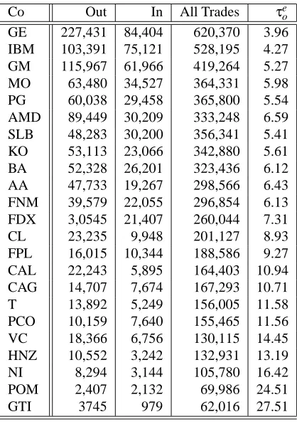
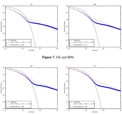
In this section we look at empirical waiting-times of 23 blue-chip companies during the period April-June 2005. Our sample of stocks includes those from Dufour and Engle (2000) that were still being traded in 2005. All data were obtained from the TAQ database made available via WRDS.

conse-quence of this is that trades that occur within the same second are recorded as if they had taken place simultaneously. On the other hand, there are cases when one trade is broken into various batches and these too are recorded as simultaneous trades. A common approach adopted in the literature has been to delete these trades. For instance, in our data set of IBM trades there are 178,512 durations of zero seconds. Deleting these observations would amount to discarding more than 28% of the 631,586 waits between trades.

Co Out In All Trades τe o

GE 227,431 84,404 620,370 3.96 IBM 103,391 75,121 528,195 4.27 GM 115,967 61,966 419,264 5.27 MO 63,480 34,527 364,331 5.98 PG 60,038 29,458 365,800 5.54 AMD 89,449 30,209 333,248 6.59 SLB 48,283 30,200 356,341 5.41 KO 53,113 23,066 342,880 5.61 BA 52,328 26,201 323,436 6.12 AA 47,733 19,267 298,566 6.43 FNM 39,579 22,055 296,854 6.13 FDX 3,0545 21,407 260,044 7.31 CL 23,235 9,948 201,127 8.93 FPL 16,015 10,344 188,586 9.27 CAL 22,243 5,895 164,403 10.94 CAG 14,707 7,674 167,293 10.71 T 13,892 5,249 156,005 11.58 PCO 10,159 7,640 155,465 11.56 VC 18,366 6,756 130,115 14.45 HNZ 10,552 3,242 132,931 13.19 NI 8,294 3,144 105,780 16.42 POM 2,407 2,132 69,986 24.51 GTI 3745 979 62,016 27.51

Table I

Empirical waiting-time data. The second column, under the heading “Out”, indicates the number of data points, for each stock, that were discarded because a zero wait was also accompanied by a zero price change. The third column, under the heading “In”, shows the number of data points which were kept

because although there was a zero wait, price changes were not zero. The fourth column indicates therefore the number of data points used as duration between trades. Finally the fifth column is the

A. Shifted-Mittag-Leffler survival function

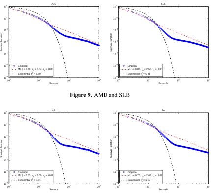
The most conspicuous message from Figure 1 is the presence of relatively ‘long’ durations. These long durations are impossible to capture with an exponential waiting-time distribution, and, as we shall see below, the presence of these long waits between trades is not unique to GM. The appendix shows 22 other companies that exhibit broadly the same shaped survival function as GM. Hence, we will justify a choice of waiting-time distribution by specifying a model that can capture the right tail of the survival function, i.e. long waits.

The first step is to observe that the shape of the right tail of the survival function, in log-log space, in Figure 1 closely resembles that of a straight line with a negative slope. It is straightforward to see that this linear behavior in a log-log plot is equivalent to observing the behavior of data that is changing with a power law. In other words the (ln-)tail of the survival function shows the behavior

lnϒ(t)_{∼ −}βln t+ln a+_···, as t _→∞, (18)

whereβ>0 and a are constants.6 Since from (1) we obtain the pdf of the waiting times by differentiating the survival function

υ(t) =₋d

dtϒ(t),

we can use (18) to find the tail behavior of the pdf of the waiting-time distribution:

lnυ(t)_{∼ −}(β+1)lnt+ln(aβ) +_···, as t_→∞. (19)

options. In addition, we would like to specify a waiting-time distribution so that expression (16) in Proposition 1 can be performed analytically.

Instead of working with the tail expression of v(t)given by (19), we look at its Laplace transform. Hence, we can write the tail of the waiting-time distribution in Laplace space as7

˜

υ(s)_∼1₋(τos)β+o(sβ), for 0<β≤1, (20)

whereτo>0 is a constant.

However, we are still left with the question of finding a suitable waiting-time distribution since we have only specified the functional form of the tail to capture the long waits. Note that there are many waiting time distributions that could exhibit a slow decay of the right tail, as shown in (20). However not all of them will deliver mathematically tractable expressions capable of being employed by standard pricing tools, and more importantly, will not facilitate the calibration of risk-neutral parameters to observed vanilla option prices (see for example Carr and Madan (1999)). Hence, below we specify v(t)for all t_≥0 by choosing a distribution function that allows us to calculate the characteristic function (16).

We proceed by noting that one possible choice of ˜υ(s), consistent with (20), is given by

˜

υ(s) = 1

1+ (τos)β

, for 0<β_≤1. (21)

Moreover, the Laplace transform of the survival function is given by

˜

ϒML(s) =

1₋υ˜(s)

s =τo

(τos)β−1

1+ (τos)β

, for 0<β_≤1, (22)

and by taking the inverse Laplace transform of (22), see equation (A7) in the appendix, the survival function becomes

ϒML(t) =

∞

∑

(₋1)j (t/τo)

βj

which is known in the literature as the Mittag-Leffler (ML), or as a generalized, exponential function. Furthermore, we make the important observation that when β= 1 the waiting-time distribution becomes the exponential with expected value E[τ] =τo. Hence, we can

view the ML survival function as a generalization of the exponential survival function that accommodates long waits between trades whenβ<1; something an exponential waiting-time distribution is unable to capture.

We employ a slight modification of (23), by including a shift parameter τs in the

time-domain of the survival function. The intuition behind this trivial modification is to recognize that the time-stamps in our data are rounded to the nearest second. Consequently the data set are left-truncated, which therefore makes it reasonable to include a shift in the domain of the survival function to improve the statistical fitting of the ML survival model. Figure 2 shows empirical and fitted survival functions. We show (shifted) ML and exponential functions. As expected, the exponential function is not capable of capturing the long waits. Moreover, Table II shows the results of fitting the shifted ML parameters to all the stocks studied here and the appendix depicts the fitted distributions.

100 101 102 103 10−6

10−5 10−4 10−3 10−2 10−1 100

GM

Seconds

Survival Function

Empirical

ML β = 0.75, τ_o = 2.08, τ_s = 0.02 Exponential τe

o = 5.27

Figure 2. Fitted survival functions for GM

A.1. European-style options with ML survival function

If we assume that, under the risk-neutral measure, the survival function has the form (21) then the problem of pricing European-style options (see Proposition 1) reduces to deriving (16). Furthermore, in this particular case, calculations get simplified if we assume that a trade just happened, i.e H(0) =0, and for simplicity we also assume that τs=0. Given the high

frequency of trade arrivals, assuming H(0) =0 is reasonable. The following Theorem shows how European-style options are priced when the survival function of the waiting times is ML.

Theorem 3 Assume that the prerequisites from Proposition 1 hold. Additionally, assume that

the survival function is ML, withτs=0, and that H(0) =0. Then the value of the European-style option is given by

V(0) =e

−rT

2π

Z ∞+iˆξ

−∞+iˆξe

−iξln S(0)_e−iξ(r−D)T_E

β,1

h

−1₋eΨ(ξ)

(T/τo)β

i

ˆ

G(ξ)dξ. (24)

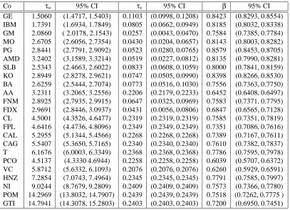
Co τo 95% CI τs 95% CI β 95% CI GE 1.5060 (1.4717, 1.5403) 0.1103 (0.0998, 0.1208) 0.8423 (0.8293, 0.8554) IBM 1.7391 (1.6934, 1.7849) 0.0805 (0.0662, 0.0949) 0.8185 (0.8032, 0.8338) GM 2.0860 ( 2.0178, 2.1543) 0.0257 (0.0043, 0.0470) 0.7584 (0.7385, 0.7784) MO 2.6705 (2.6056, 2.7354) 0.0430 (0.0204, 0.0657) 0.8143 (0.8003, 0.8282) PG 2.8441 (2.7791, 2.9092) 0.0523 (0.0280, 0.0765) 0.8579 (0.8453, 0.8705) AMD 3.2402 (3.1589, 3.3214) 0.0519 (0.0227, 0.0812) 0.8135 (0.7990, 0.8281) SLB 2.5343 (2.4663, 2.6022) 0.0833 (0.0608, 0.1059) 0.8000 (0.7841, 0.8159) KO 2.8949 (2.8278, 2.9621) 0.0747 (0.0505, 0.0990) 0.8398 (0.8266, 0.8530) BA 2.6259 (2.5444, 2.7074) 0.0773 (0.0516, 0.1030) 0.7556 (0.7363, 0.7750) AA 3.2311 (3.2065, 3.2556) 0.2206 (0.2179, 0.2233) 0.6452 (0.6408, 0.6497) FNM 2.8925 (2.7935, 2.9915) 0.0647 (0.0325, 0.0969) 0.7583 (0.7371, 0.7795) FDX 2.9691 (2.8446, 3.0937) 0.0431 (0.0056, 0.0806) 0.6847 (0.6565, 0.7128) CL 4.5001 (4.3526, 4.6477) 0.2319 (0.2319, 0.2319) 0.7585 (0.7351, 0.7819) FPL 4.6416 (4.4736, 4.8096) 0.2349 (0.2349, 0.2349) 0.7351 (0.7086, 0.7616) CAL 5.2955 (5.1344, 5.4566) 0.2268 (0.2268, 0.2268) 0.7389 (0.7167, 0.7611) CAG 5.5407 (5.3650, 5.7165) 0.2340 (0.2340, 0.2340) 0.7610 (0.7382, 0.7837) T 6.1676 (6.0003, 6.3349) 0.2368 (0.2368, 0.2368) 0.7786 (0.7595, 0.7978) PCO 4.5137 (4.3330 4.6944) 0.2258 (0.2258, 0.2258) 0.6039 (0.5707, 0.6372) VC 5.8712 (5.6332, 6.1093) 0.2076 (0.2076, 0.2076) 0.6260 (0.5929, 0.6591) HNZ 7.2854 (7.0743, 7.4964) 0.2345 (0.2345, 0.2345) 0.7791 (0.7585, 0.7997) NI 9.0244 (8.7679, 9.2809) 0.2409 (0.2409, 0.2409) 0.7573 (0.7366, 0.7780) POM 14.2969 (13.8032, 14.7907) 0.2439 (0.2439, 0.2439) 0.7518 (0.7262, 0.7775 ) GTI 14.7941 (14.3078, 15.2803) 0.2403 (0.2403, 0.2403) 0.7200 (0.6950, 0.7451)

Table II

Shifted ML parameter estimates forτo,τs(in seconds) andβusing ultra-high-frequency data for the trading period April 1st through June 30th 2005.

Regarding the choice of ˆξ in the integration limits in Theorem 3, we require

E_β,1h₋1₋eΨ(ξ)(T/τo)β

i

to be analytic in a strip that intersects the strip where the (com-plex) Fourier transform of the G(_·)exists. The ML function (A6) is an entire function; there-fore it is analytic where eΨ(−ξ) is analytic. Thus, the restrictions on ˆξare the same as those required in the particular case whenβ=1, i.e. when pricing with L´evy processes.8 For exam-ple, if we let β=1, we can verify that the price of a European call option with strike K and maturity T , using (24), is given by

V(0; K,T) =₋e−

rT_K

2π

Z ∞+iˆξ

−∞+iˆξe

−iξln S(0)+T_[−iξ(r−D)+(Ψ(−ξ)−1)τ−1

o ] K iξ

ξ2_−iξdξ,

IV. Estimation of risk-neutral parameters

In this section we present results obtained from calibrating risk-neutral parameters to IBM option prices. We obtained data for traded American options written on IBM. This data set include the spot price, strike, maturity, implied volatility, dividend yield and interest rate. We used the parameters from the American options to devise a new data set of European options. We then used the algorithm employed in Carr and Wu (2003) to estimate the risk-neutral parameters of our model by considering two cases. In the first we assume that price revisions possess a Gaussian distribution and that the waiting-time survival function is the ML function. In the second case we still assume that the waiting-time survival function is the ML function but now assume that price revisions possess an FMLS distribution (Carr and Wu (2003)).

The tables in Appendix C show the results for every trading day from April 1 through May 6 2005. In any given day we have IBM options for different strikes and for different maturities. We show the results of the calibration for the lot of IBM options with shortest maturity (including all strikes), then we add to these results the next lot, which includes those options with second shortest maturity, and so on.10 For example, the first row in Table C shows risk-neutral parameters obtained from 6 options that expired in 10 working days (i.e. the first lot). For this lot, the resulting volatility of Gaussian price revisions and the beta of the model areσ=0.00058 andβ=0.717300 respectively, and for FMLS price revisions α=1.99, σ=0.000318 and β=0.72004.11 In the second row, we show the results of the calibration procedure when we take into account the options that expire between 10 and 35 working days.

parameter β could be accommodating for kurtosis of the risk-neutral distribution which, is produced by the spatial shocks, and is ‘picked up’ by the parameter β. In the next section we see how the presence of long durations (β<1) increases the kurtosis of the risk-neutral distribution of spot prices.

V. Numerical examples: the impact of waiting times on

op-tion prices

In the previous section, we looked at the calibration of risk-neutral parameters for models that explicitly include waiting times between trades. Here, to gain more insight into the conse-quences of including durations, we present two examples of how waiting times affect option prices. These are calculated by choosing plausible risk-neutral parameters, so that we can focus on the effects of assuming the ML survival function. The first example assumes that the spatial shocks are Gaussian and the second example assumes that spatial shocks possess a CGMY distribution (see Carr, Geman, Madan, and Yor (2002)). In all examples we assumed that τo=1/1,200,000, (i.e. that there are, on average, 100,000 trades per month) and that

τs=0.

A. Gaussian price revisions and ML waiting-times

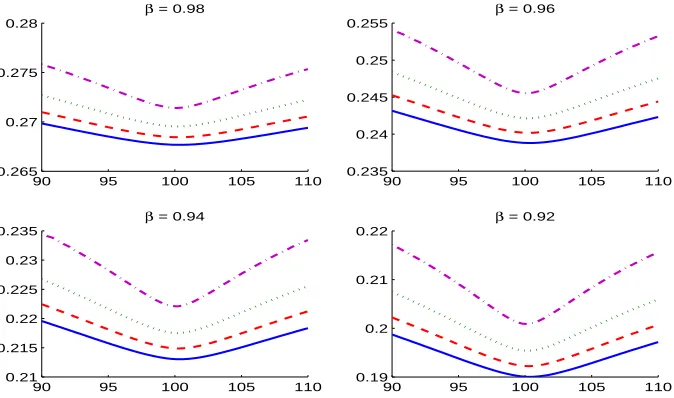
Figure 3 shows implied volatility (IV) when it is assumed that spatial shocks are Gaussian with mean zero and volatilityσ=0.3√τo. With this choice of volatility, and lettingβ=1, the

model is asymptotically equivalent to assuming a Black-Scholes model with volatilityσBS=

that are not exponential, gives rise to the commonly observed convexity of the IV in the Black-Scholes framework despite the fact that spatial shocks are Gaussian.12 Note that the waiting time affects the convexity of the IV in a symmetric way and does not reproduce smirks or skewed IVs. In our framework, market participants include a premium, over and above the classical Black-Scholes price for out-of-the-money values, to price in the duration times be-tween trades.

Another important feature of Figure 3 is the fact that the IV range decreases asβdecreases. For example, when β=0.98 and expiry is T =20 days, IV is roughly within [0.265,0.27]

whereas whenβ=0.94 and T=20, IV is in the range[0.21,0.22]. This result is not surprising, and is in line with the findings of Engle (2000) and Dufour and Engle (2000). Indeed in our model, the market will exhibit less activity (understood here as number of trades over a time period) and lower IV the lower βis. This is also clear in Figure 4 where, still with Gaussian spacial shocks, we fix expiry dates and vary β=_{1,0.98,0.96,0.94,0.92_}where the exponential case is included.

90 95 100 105 110 0.265

0.27 0.275 0.28

β = 0.98

90 95 100 105 110 0.235

0.24 0.245 0.25 0.255

β = 0.96

90 95 100 105 110 0.21

0.215 0.22 0.225 0.23 0.235

β = 0.94

90 95 100 105 110 0.19

0.2 0.21 0.22

β = 0.92

Figure 3. Implied Volatility across strike for conditionally Gaussian model with waiting times for β=

{0.98,0.96,0.94,0.92_}. The volatility of the zero-mean Gaussian price revisions areσ=0.3√τo, and the pa-rameters for option pricing are r=5%, D=0 and S0=100. The dash-dotted line corresponds to T =5 days,

90 95 100 105 110 0.2

0.25 0.3 0.35

T = 20 days

90 95 100 105 110 0.2

0.25 0.3 0.35

T = 15 days

90 95 100 105 110 0.2

0.25 0.3 0.35

T = 10 days

90 95 100 105 110 0.2

0.25 0.3 0.35 0.4

T = 5 days

Figure 4. Implied Volatility across strike for conditionally Gaussian with waiting times for different days to maturity T={20,15,10,5_}and varyingβ={1,0.98,0.96,0.94,0.92_}. The volatility of the zero-mean Gaussian price revisions areσ=0.3√τo, and the parameters for option pricing are r=5%, D=0 and S0=100, and the

parameters for option pricing are r=5%, D=0 and S0=100. Each panel shows how implied volatility varies

when expiry remains fixed andβvaries. The solid line representsβ=1, the dashed line corresponds toβ=0.98, the dotted line corresponds toβ=0.96, the dash-dotted line corresponds toβ=0.94, and circles corresponds to

β=0.92.

B. CGMY price revisions and ML waiting-times

In this subsection we produce the same results as above, but we allow the distribution of price revisions to exhibit fatter tails than the Gaussian distribution by choosing price revisions with a a CGMY distribution, see Carr, Geman, Madan, and Yor (2002). In our examples below, we assumed that C=1.8750_×10−7, Y =1.5, G=10, M=20, this implies that the distribution of the spatial shocks has negative asymmetry because G<M, and both the left and right tails

90 95 100 105 110 0.2

0.25 0.3 0.35 0.4

β = 0.98

90 95 100 105 110 0.2

0.25 0.3 0.35 0.4

β = 0.96

90 95 100 105 110 0.2

0.25 0.3 0.35

β = 0.94

90 95 100 105 110 0.2

0.25 0.3 0.35

β = 0.92

90 95 100 105 110 0.2

0.25 0.3 0.35

T = 20 days

90 95 100 105 110 0.2

0.25 0.3 0.35

T = 15 days

90 95 100 105 110 0.2

0.25 0.3 0.35

T = 10 days

90 95 100 105 110 0.2

0.25 0.3 0.35 0.4

T = 5 days

Figure 6. Implied Volatility across strike for CGMY with waiting times for different days to maturity T =

{20,15,10,5_}and varyingβ={1,0.98,0.96,0.94,0.92_}. Each panel shows how implied volatility varies when expiry remains fixed andβvaries. The solid line representsβ=1, the dashed line corresponds toβ=0.98, the dotted line corresponds toβ=0.96, the dash-dotted line corresponds to β=0.94, and circles corresponds to

β=0.92.

VI. Conclusions

Until now, the financial literature has only considered the question of how waiting-times or duration between trades affect the dynamics of stock prices. The question of how this random duration affects derivative prices, has not previously been addressed. In this article we propose a model that explicitly incorporates these waiting-times. Besides capturing duration between trades, our model also captures key behavioral characteristics recorded in the empirical litera-ture such as the non-Markovianity of stock prices, Easley and O’Hara (1992).

We propose the use of the ML survival function as a candidate to model waiting times. One of the main advantages is that with the ML it is straightforward to use the usual transform methods employed in the L´evy process literature relating to finance to price options. As an example, we calibrated risk-neutral parameters, using IBM options data, to a model with ML waits and Gaussian price revisions and to a model with ML waits and FMLS price revisions. In both cases the effects of durations were captured by risk-neutralβs, which were in the vast majority of cases less than one.

References

A¨ıt-Sahalia, Yacine, and Per A. Mykland, 2003, The Effects of random and discrete sampling when

estimating continuous-time diffusions, Econometrica 71, 483–549.

Cameron, A. Colin, and Pravin K. Trivedi, 1996, Count data models for financial data, in G.S. Maddala,

and Calyampudi Rao, eds.: Handbook of Statistics (Elsevier, North-Holland, Amsterdam, ).

Carr, Peter, Hellyete Geman, Dilip Madan, and Marc Yor, 2002, The fine Structure of asset returns: an

empirical investigation, Journal of Business 75, 305–332.

Carr, Peter, and Dilip Madan, 1999, Option Valuation Using the Fast Fourier Transform, Journal of

Computational Finance 2, 61–73.

Carr, Peter, and Liuren Wu, 2003, The Finite Moment Logstable Process and Option Pricing, The

Journal of Finance LVIII, 753–777.

Carr, Peter, and Liuren Wu, 2004, Time-Changes L´evy Processes and Option Pricing, Journal of

Fi-nancial Economics 71, 113–141.

Cont, Rama, and Peter Tankov, 2004, Financial Modelling With Jump Processes. (Chapman and Hall

London) 1st edn.

Diamond, Douglas W., and Robert E. Verrechia, 1987, Constraints on short-selling and asset price

adjustment to private information, Journal of Financial Economics 18, 277–311.

Dufour, Alfonso, and Robert F. Engle, 2000, Time and the Price Impact of a Trade, The Journal of

Finance LV, 2467–2498.

Easley, David, and Maureen O’Hara, 1992, Time and the Process of Security Price Adjustment, The

Journal of Finance XLVII, 577–605.

Engle, Robert F., 2000, The Econometrics of Ultra-High-Frequency Data, Econometrica 68, 1–22.

Engle, Rober F., and Jeffrey R. Russell, 1998, Autoregressive Conditional Duration: A New Model for

Jacobsen, Martin, 2006, Point Process Theory and Applications. (Birkh¨auser).

Jacod, Jean, and Albert N. Shiryaev, 2002, Limit Theorems for Stochastic Processes vol. 228 of A

Series of Comprehensive Studies in Mathematics. (Springer).

Mainardi, Francesco, Marco Raberto, Rudolg Gorenflo, and Enrico Scalas, 2000, Fractional Calculus

and Continuous-time Finance II: the waiting-time distribution, Physica A 287, 469–481.

Podlubny, Igor, 1999, Fractional Differential Equations vol. 198 of Mathematics in Science and

Appendix A. Proofs of propositions and the ML function

Proof Theorem 1.

We show that(X(t),H(t))is described by a stochastic differential equation (SDE), whose

coeffi-cients only depend on the process itself. Then it is well known that(X(t),H(t))is a time homogenous

Markov process.

In between trades, the backward recurrence time H(t)defined in (6) evolves linearly in t and reverts

to zero each time there is a jump in X(t). Therefore H(t)follows the dynamics given by the SDE

dH(t) =dt−H(t−)dNt =dt− Z

R0

H(t−)z N1(dt,dz).

where N1(ω,dt,dz) =N1(dt,dz)denotes the integer valued random measure that represents the jump

measure of the counting process Nt. The intensity of the counting process Nt is given by u(H(t))(see

e.g. Jacobsen (2006)) where the hazard function u(t) is given by (2). We can write the predictable

compensating measure of N1(dt,dz)as

ν1_{(ω,dt,dz) =u(H(t))dtδ}

1(dz), (A1)

whereδ1(dz)is the Dirac measure centered at 1.

Then it follows that the multivariate dynamics of the two-dimensional process (X(t),H(t))is

de-scribed by

dX(t)

dH(t)

=

r₋D

1 dt+   1 0

0 ₋H(t−)





dX(t)

dN(t)

(A2)

=

r₋D

1 dt+ Z R2 0 z1

−H(t−)z2

N2(dt,dz1,dz2)

where N2(ω,dt,dz1,dz2) =N2(dt,dz1,dz2)denotes the jump measure of the two-dimensional process

but with independently distributed jump sizes, the predictable compensator of N2(dt,dz1,dz2)is given

by

ν2_(ω,dt,dz

1,dz2) =u(H(t))g(z1)dtdz1δ1(dz2). (A3)

Thus the two-dimensional process (X(t),H(t))is described by SDE (A2) with Lipschitz continuous

coefficients and predictable compensator that only depend on the process(X(t),H(t))itself (more

pre-cisely, on the second component H(t)). Then it is well known that(X(t),H(t))is a time-homogenous

Markov process.

Proof Proposition 1.

We will denote the Fourier transform of a function g(x)by

F [g(x)] =gˆ(ξ) =

Z ∞

−∞e

ixξ_g(x)dx,

whereξ∈C. Hence, assuming the pay-off G(_·)is such that we can invert its Fourier transform,

V(t) = e−r(T−t)EQ[G(X(T))_|Ft]

= e−r(T−t)EQ

1

2π

Z ∞+iξi

−∞+iξi

e−iξXT_Gˆ₍ξ_)dξ_|F

t

= e−

r(T−t)

2π

Z ∞+iξi

−∞+iξi

e−iξln S(t)e−iξ(r−D)(T−t)EQ

h

eiξ∑NTi=Nt+1Yi_|F

t i

ˆ

G(ξ)dξ, (A4)

whereEQdenotes the risk-neutral expectation operator.

Proof Theorem 3.

We will denote the Laplace transform of a function f(t)by

L[f(t)] = ˜f(s) =

Z ∞

0

Further, we assume H(0) =0, i.e. a trade just happened. It will be useful to have an expression for

the probability density function P(n,t)of observing n trades during the time interval [0,t]. Using the

survival function (1) the probability that a trade does not take place before time t is given by

P(n=1,t) =

Z t

0 υ

(s)ϒ(t₋s)ds= (υ⋆ϒ)(t),

where⋆denotes convolution. Then the probability of observing n trades over the interval[0,t]is given

by(υn_{⋆ϒ)(t)and taking its Laplace transform yields}

˜

P(n,s) =υ˜(s)nϒ˜(s) =υ˜(s)n1−υ˜(s)

s . (A5)

Therefore, from Proposition 1, we need to calculate

ˆ

q(ξ,0,T) = EQ

h eiξ∑NTi=1Yi

i

= EQ

h

e(NT)Ψ(ξ)

i

L_{qˆ(ξ,0,T)_} = L n

EQ

h

e(NT)Ψ(ξ)

io

= L

(_∞

∑

0

P(n,T)enΨ(ξ) )

=

∞

∑

0

L_{P(n,T)_}enΨ(ξ)

=

∞

∑

0 ˜

P(n,s)enΨ(ξ)

=

∞

∑

0 ˜

υ(s)n1−υ˜(s)

s e

nΨ(ξ)

= 1−υ˜(s)

s

∞

∑

0 ˜

υ(s)nenΨ(ξ)

= 1−υ˜(s)

s

1 1₋eΨ(ξ)υ_˜(s).

where ˜υis given by (21). Then

ˆ

q(₋ξ,0,T) = L−1

1₋υ˜(s)

s

1 1−eΨ(−ξ)υ˜(s)

= E_β,1h₋1₋eΨ(−ξ)(T/τo)β i

The ML function

In its most general form, the two-parameter Mittag-Leffler function is given by

E_β,γ(z) =

∞

∑

j=0 zj

Γ(βj+γ), β>0, γ>0. (A6)

and its Laplace transform, see Podlubny (1999), by

L n

tβn+γ−1E_β(n_,γ)(_±atβ)o= n!s

β−γ

(sβ_∓a)n+1, Re(s)>|a|

1/γ_{, (A7)}

where E_β(n_,γ)(y) = _dydnnEβ,γ(y). This distribution has previously been proposed in the context of financial

Appendix B. Empirical and fitted Shifted-Mittag-Leffler

sur-vival function

100 ₁₀1 ₁₀2 ₁₀3

10−6 10−5 10−4 10−3 10−2 10−1 100 GE Seconds Survival Function Empirical

ML β = 0.84, τo = 1.50, τs = 0.11 Exponential τe

o = 3.96

100 ₁₀1 ₁₀2 ₁₀3

10−6 10−5 10−4 10−3 10−2 10−1 100 IBM Seconds Survival Function Empirical

ML β = 0.81, τo = 1.73, τs = 0.08 Exponential τe

o = 4.27

Figure 7. GE and IBM

100 101 102 103

10−6 10−5 10−4 10−3 10−2 10−1 100 MO Seconds Survival Function Empirical

ML β = 0.81, τ_o = 2.67, τ_s = 0.04 Exponential τe

o = 5.98

100 101 102 103

10−6 10−5 10−4 10−3 10−2 10−1 100 PG Seconds Survival Function Empirical

ML β = 0.85, τ_o = 2.84, τ_s = 0.05 Exponential τe

o = 5.54

100 101 102 103 10−6 10−5 10−4 10−3 10−2 10−1 100 AMD Seconds Survival Function Empirical

ML β = 0.76, τ_o = 2.64, τ_s = 0.05 Exponential τe

o = 6.59

100 101 102 103

10−6 10−5 10−4 10−3 10−2 10−1 100 SLB Seconds Survival Function Empirical

ML β = 0.80, τ_o = 2.53, τ_s = 0.08 Exponential τe

o = 5.41

Figure 9. AMD and SLB

100 ₁₀1 ₁₀2 ₁₀3

10−6 10−5 10−4 10−3 10−2 10−1 100 KO Seconds Survival Function Empirical

ML β = 0.83, τo = 2.89, τs = 0.07 Exponential τe

o = 5.61

100 ₁₀1 ₁₀2 ₁₀3

10−6 10−5 10−4 10−3 10−2 10−1 100 BA Seconds Survival Function Empirical

ML β = 0.75, τo = 2.62, τs = 0.07 Exponential τe

o = 6.12

100 101 102 103 10−6 10−5 10−4 10−3 10−2 10−1 100 AA Seconds Survival Function Empirical

ML β = 0.81, τ_o = 3.24, τ_s = 0.05 Exponential τe

o = 6.43

100 101 102 103

10−6 10−5 10−4 10−3 10−2 10−1 100 FNM Seconds Survival Function Empirical

ML β = 0.75, τ_o = 2.89, τ_s = 0.06 Exponential τe

o = 6.13

Figure 11. AA and FNM

100 ₁₀1 ₁₀2 ₁₀3

10−6 10−5 10−4 10−3 10−2 10−1 100 FDX Seconds Survival Function Empirical

ML β = 0.68, τo = 2.96, τs = 0.04 Exponential τe

o = 7.31

100 ₁₀1 ₁₀2 ₁₀3

10−6 10−5 10−4 10−3 10−2 10−1 100 CL Seconds Survival Function Empirical

ML β = 0.75, τo = 4.50, τs = 0.23 Exponential τe

o = 8.93

100 101 102 103 10−6 10−5 10−4 10−3 10−2 10−1 100 FPL Seconds Survival Function Empirical

ML β = 0.73, τ_o = 4.64, τ_s = 0.23 Exponential τe

o = 9.27

100 101 102 103

10−6 10−5 10−4 10−3 10−2 10−1 100 CAL Seconds Survival Function Empirical

ML β = 0.73, τ_o = 5.29, τ_s = 0.22 Exponential τe

o = 10.94

Figure 13. FPL and CAL

100 ₁₀1 ₁₀2 ₁₀3

10−6 10−5 10−4 10−3 10−2 10−1 100 CAG Seconds Survival Function Empirical

ML β = 0.76, τo = 5.54, τs = 0.23 Exponential τe

o = 10.71

100 ₁₀1 ₁₀2 ₁₀3

10−6 10−5 10−4 10−3 10−2 10−1 100 T Seconds Survival Function Empirical

ML β = 0.77, τo = 6.16, τs = 0.23 Exponential τe

o = 11.58

100 101 102 103 10−6 10−5 10−4 10−3 10−2 10−1 100 PCO Seconds Survival Function Empirical

ML β = 0.60, τ_o = 4.51, τ_s = 0.22 Exponential τe

o = 11.56

100 101 102 103

10−6 10−5 10−4 10−3 10−2 10−1 100 VC Seconds Survival Function Empirical

ML β = 0.62, τ_o = 5.87, τ_s = 0.20 Exponential τe

o = 14.45

Figure 15. PCO and VC

100 ₁₀1 ₁₀2 ₁₀3

10−6 10−5 10−4 10−3 10−2 10−1 100 HNZ Seconds Survival Function Empirical

ML β = 0.77, τo = 7.28, τs = 0.23 Exponential τe

o = 13.19

100 ₁₀1 ₁₀2 ₁₀3

10−6 10−5 10−4 10−3 10−2 10−1 100 NI Seconds Survival Function Empirical

ML β = 0.75, τo = 9.02, τs = 0.24 Exponential τe

o = 16.42

100 101 102 103 10−6

10−5 10−4 10−3

10−2

10−1 100

POM

Seconds

Survival Function

Empirical

ML β = 0.75, τ_o = 14.29, τ_s = 0.24 Exponential τe

o = 24.51

100 101 102 103

10−6 10−5 10−4 10−3

10−2

10−1 100

GTI

Seconds

Survival Function

Empirical

ML β = 0.72, τ_o = 14.79, τ_s = 0.24 Exponential τe

o = 27.51

Gaussian Revisions FMLS Revisions

Date Days to Expiry N σ β α σ β

Gaussian Revisions FMLS Revisions

Date Days to Expiry N σ β α σ β

Gaussian Revisions FMLS Revisions

Date Days to Expiry N σ β α σ β

Gaussian Revisions FMLS Revisions

Date Days to Expiry N σ β α σ β

29-Apr 15 6 0.000657 0.735341 2.000 0.000581 0.697424 15, 34 17 0.000225 0.920759 1.963 0.000139 0.922504 15, 34, 53 33 0.000188 0.951725 1.942 0.000110 0.949275 15, 34, 53, 122 50 0.000248 0.906644 1.930 0.000147 0.896451 15, 34, 53, 122, 165 80 0.000238 0.912866 1.911 0.898226 0.912866 02-May 14 5 0.011543 0.259218 1.919 0.004782 0.325828 14, 33 18 0.000343 0.853764 1.881 0.000154 0.862809 14, 33, 52 35 0.000285 0.886290 1.885 0.000139 0.882137 14, 33, 52, 121 52 0.000268 0.896363 1.878 0.000139 0.878174 14, 33, 52, 121, 164 82 0.000253 0.905821 1.868 0.000129 0.883145 03-May 13 5 0.001237 0.622567 1.955 0.005310 0.687560 13, 32 16 0.000294 0.871768 1.940 0.000170 0.871658 13, 32, 51 32 0.000203 0.935920 1.916 0.000109 0.931191 13, 32, 51, 120 49 0.000210 0.930860 1.905 0.000116 0.915789 13, 32, 51, 120, 163 79 0.000197 0.940805 1.887 0.000105 0.920991 04-May 12, 31 15 0.000201 0.931271 1.931 0.000121 0.918467 12, 31, 50 32 0.000153 0.979814 1.907 0.000084 0.964831 12, 31, 50, 119 49 0.000186 0.947142 1.895 0.000104 0.925190 12, 31, 50, 119, 162 79 0.000183 0.950338 1.881 0.000098 0.925661 05-May 11, 30 14 0.000155 0.976139 1.919 0.000101 0.943334 11, 30, 49 30 0.000137 0.999998 1.901 0.000073 0.985243 11, 30, 49, 118 47 0.000178 0.957262 1.892 0.000102 0.928288 11, 30, 49, 118, 161 77 0.000161 0.970512 1.880 0.000100 0.923934 06-May 10 9 0.027844 0.095816 1.600 0.003676 0.253083 10, 29 22 0.000390 0.825186 1.667 0.000117 0.772995 10, 29, 48 39 0.000224 0.922345 1.720 0.000083 0.858699 10, 29, 48, 117 56 0.000236 0.914281 1.743 0.000098 0.848417 10, 29, 48, 117, 160 86 0.000236 0.914281 1.772 0.000097 0.867299

Table III

Notes

1_{Below we discuss in detail how consolidated trades from the TAQ database were}

em-ployed.

2_{In fact, a Kolmogorov-Smirnov test clearly rejects the hypothesis that the data came from}

an exponential survival function.

3_{In the language of counting processes the process∑}Nt

i=1Yi is called a (0-delayed) renewal

process.

4_{Likewise in most stochastic volatility models where the volatility factor under the}

risk-adjusted measure is essentially the same under the physical measure, but with a linear adjust-ment.

5_{We calculate this arbitrary duration strictly greater than zero in the following way. Out}

of all the zero-duration trades we count how many times there were two trades within one second, three trades within one second, etc. Then we calculate a weighted average of number of trades within one second and assume that these occur within 0.5 second instead of deleting them from the sample. Furthermore, for simplicity we do not alter the duration of the trade following those zero-duration trades for which we assigned a non-negative duration.

6_{The constant a could be a function of the parameterβ.} 7_{To arrive at expression (20) we use the property that}

L

L

−dϒ(t)

dt

=₋sL_{at−β_}+ϒ(0) =₋aγ(1₋β)sβ+1,

and restrict 0<β_≤1 to have a valid (monotonic) survival function.

8_{There are a number of articles in the literature that use transform techniques to price and}

9_{Note that we must require e}Ψ(−ξ) _{to be analytic in a line that intersects[−∞+iˆξ,∞+iˆξ]}

where ˆξ>1.

10 _{We do not calibrate to lots where there are less than 5 options.}

11_{For simplicity we assumed thatτ}

oremained the same under both the physical and

statis-tical measure (see Table II for IBM) and thatτs=0.

12_{Figure 3 does not include the case} β_{=1 where IV becomes 0.30 for all expiries as}