BIROn - Birkbeck Institutional Research Online
Robertson, D. and Wright, Stephen (2009) The limits to stock return
predictability. Working Paper. Birkbeck, University of London, London, UK.
Downloaded from:
Usage Guidelines:
Please refer to usage guidelines at or alternatively
The Limits to Stock Return Predictability
∗
Donald Robertson and Stephen Wright
†September 10, 2009
Abstract
We examine predictive return regressions from a new angle. We ask what observable
univariate properties of returns tell us about the “predictive space” that defines the true predictive model: the triplet¡λ, R2x, ρ¢,where λis the predictor’s persistence, R2x is the
predictive R-squared, and ρis the "Stambaugh Correlation" (between innovations in the
predictive system). When returns are nearly white noise, and the variance ratio slopes
downwards, the predictive space can be tightly constrained. Data on real annual US stock
returns suggest limited scope for even the best possible predictive regression to out-predict
the univariate representation, particularly over long horizons.
Keywords: Predictive return regressions, variance ratio, fundamental and non-fundamental univariate representations.
∗We are grateful for comments from Kenneth French, Andrew Harvey, Alan Timmerman and Ron Smith.
†Faculty of Economics, University of Cambridge, [email protected]and Dept of Economics,
1
Introduction
A perennial problem in empiricalfinance is the question of whether it is possible to predict stock
market returns using some predictor variable. In addition to the question of what predictor
variable to use (the list of potential predictors includes, inter alia, dividend yields, interest
rates, book-market values, price-earnings ratios), there are econometric questions regarding the
appropriate distributional theory for inference (Stambaugh 1999, Campbell and Yogo 2006, Ang
and Bekaert 2006 and many others); whether any underlying relationships are stable enough
to allow useful predictability, or may simply arise from data mining (Pesaran and Timmerman
1995, Timmermann and Paye 2006, Ferson et al 2003, Goyal and Welch 2003, Campbell and
Thomson 2008, Cochrane 2008a); and whether observable predictors may be at best imperfect
proxies for the true predictor (Pastor & Stambaugh, 2009). Finally there is a closely related
literature that addresses differences between one period ahead and long horizon regressions (see
for example Campbell and Viceira 2002; Cochrane, 2008a; Boudoukh et al, 2008).
In this paper we examine predictive return regressions from a new angle. It is well-known
that when one time series predicts another the properties of the predictive system (including
the univariate properties of the predictor variable) determine the univariate properties of the
predicted variable (in this case returns).1 But we can also view the process in reverse. In this
paper we ask what the observable univariate properties of returns tell us about the “predictive
space” that defines the true predictive model: the triplet (λ, R2
x, ρ) where λ is the
predic-tor’s persistence, R2x is the predictive R2, and ρ is the "Stambaugh Correlation" (between the
innovations to the predictor autoregression and those in the predictive return regression ).2
If these insights depended on tight estimates of parameters in an ARMA representation
our analysis would not be of much practical value. But in fact the reverse is the case. The
very fact that ARMA representations of returns fit so poorly is informative about the nature
of the predictive space for predictive models in general. But a second feature of returns data
1Note that we are assuming that the predictor is, in Pastor & Stambaugh’s (2009) terminology, a "perfect predictor", ie one that captures "true" expected returns, and hence, up to a white noise expectational error, also generates the actual data for returns.
also has potentially very significant implications for the predictive space: whether the variance
ratio of long-horizon returns slopes downwards. The academic literature that directly tests for
this latter feature has not yielded unanimous conclusions (contrast, for example, the orginal
evidence presented by Poterba and Summers 1988 with the revisionist approach of,eg,Kim et
al 1991. But we would argue that the implications of what we term “variance compression”3
are worth considering, first, because it is usually taken for granted (whether explicitly or
im-plicitly) by investment practioners as the basis for the buy-and-hold strategy (for the classic
explicit statement of this view see Siegel, 1998); and second, because the analysis we present
in this paper will lead us to argue that it is also implicit in a much wider range of literature
that assumes predictability of returns, especially over long horizons (for example, Campbell &
Viceira 2002, Cochrane, 2008a).
Since a declining variance ratio is a univariate property it cannot co-exist with returns being
completely unpredictable from their own past, although we show that there is no necessary
contradiction between a quite significantly declining variance ratio at long investor horizons
and a very weak degree of short-term univariate predictability. However, the combination of
these two features does have significant implications for the predictive space that contains
all logically possible true predictive regressions. We show that the predictive space for stock
returns can quite easily contract to such an extent that there is little, if any, scope for predictive
regressions to out-predict the univariate representation, particularly at long horizons.
Recent stock market movements have been a reminder of the continuing significance of this
issue. Many predictors of stock returns originate as valuation indicators. In the late 1990s most
were signalling that the market was “over-valued”, in the very broad sense of the word4 that
such indicators were predicting weak returns (see, for example, Campbell & Shiller, 1998;Shiller,
2000; Fama & French, 2002). In the more recent past, as markets have weakened sharply, the
issue has arisen of when they become sufficiently “cheap” to offer a good prospect of unusually
strong returns. Most such indicators can be interpreted as the ratio of the stock price to some
3For reasons noted below we prefer this term to the more commonly used “mean reversion”, which a) is not always consistently defined by different authors; and b) we argue can be a misnomer.
estimate of the underlying fundamental. Our analysis suggests that even if the best possible
measure of the fundamental were found, its price ratio might barely predict any better than
simply using the history of returns to forecast future returns.
The paper proceeds as follows.
We first, in Section 2, briefly summarise the evidence for the two key empirical features of
stock returns that motivate our analysis: a low univariate R2 and a declining variance ratio.
We then show, in Section 3, the links between the standard predictive regression framework
and the univariate representation of returns.
Our key results are in Section 4, where we show how observable univariate properties of
returns can restrict the predictive space. We show that we show that we can derive lower
and upper bounds for the predictiveR2 of the true predictor that depend solely on univariate
properties.5 We then show that a declining variance ratio for long-horizon returns implies that
the Stambaugh Correlation,ρ,is in general bounded away from zero, and for a plausible range
of ARMA parameters can be close to unity. A high Stambaugh Correlation is usually treated as
a nuisance that complicates inference; we show that it is an intrinsic characteristic of the true
predictor of stock returns if there is variance compression.6 Finally we show a further feature
that arises from these restrictions on the predictive space: the correlation between the true
predictor and a “pseudo predictor”, derived solely from the history of returns, is also bounded
away from zero. It approaches unity as the predictive space contracts; however even when the
predictive space is quite tightly constrained this correlation can still be some way below unity.
In Section 5 we provide an empirical illustration. Point estimates derived from estimated
ARMA representations of returns suggest that the predictive space is very tightly constrained.
5The sole case in which this result lacks any content arises if the predictor has persistenceλ= 0,and returns are white noise. In this limiting case the predictor may predict as poorly as the ARMA representation (ie, have anR2 of zero) or (in the limit) perfectly, with an R2 of unity (albeit in the latter case only if by divine
dispensation, if the predictor this year is simply next year’s return). But in all other cases the bounds are non-trivial, in the sense that either upper or lower bound, or both, lie strictly between zero and unity.
The estimate of the best possible predictiveR2 of any possible predictor is around 10%, and of
the minimum absolute Stambaugh Correlation is at least 0.9. The implied lower bound for the
correlation between the best possible predictor and the “pseudo predictor” is lower, but still a
long way from zero. These estimates therefore suggest limited scope for even the best possible
predictor of returns to out-perform the univariate representation.
Given the imprecision of ARMA estimation, we acknowledge that a quite wide range of
near-white noise processes could also be generating the return series, for some of which the
pre-dictive space is less constrained. However, a key requirement for a significantlyless constrained
predictive space is that the true predictor must have quite low persistence. Our analysis
there-fore suggests two simple pre-tests for potential predictors of stock returns: they should not look
too similar to the “pseudo predictor” that summarises the history of returns; and they should
not be too persistent. It is notable that few, if any, commonly used predictors of stock returns
match up to either of these criteria.
Finally, in Section 6 we note a further implication of our analysis for the the predictability
literature. The strength of long-horizon return predictability is driven by a combination of
predictor persistence and a declining variance ratio; but it is exactly these features that lead
to a tightly restricted predictive space. It therefore follows that significant long-horizon return
predictability, if it exists, must be close to being a univariate phenomenon.
In Section 7 we draw conclusions and implications of our analysis; appendices provide
algebraic derivations and proofs.
2
Univariate features of returns
Wefirst briefly summarise the observable features of returns that we shall draw on in the rest
of the paper.
2.1
Returns are near-white noise
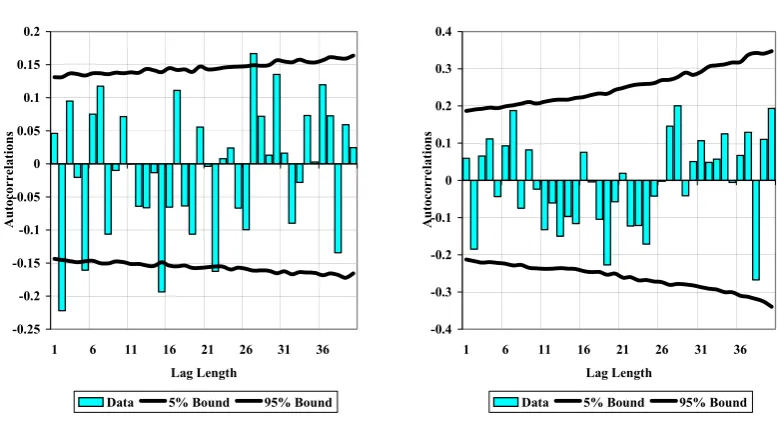
In Figure 1 we show the autocorrelation function for real annual stock returns in the United
a reasonably consistent basis for a broad based US stock market measure (the Cowles (1938)
industrial index from 1871-1925, and the S&P 500 thereafter).7 The shorter sample allows for
the possibility that return properties may have changed in the postwar era (consistent with the
[image:7.595.92.482.214.430.2]claims discussed below by Kim et al, 1991).
Figure 1. The Autocorrelation Function of Real US Stock Returns
1871-2008
-0.25 -0.2 -0.15 -0.1 -0.05 0 0.05 0.1 0.15 0.2
1 6 11 16 21 26 31 36 Lag Length
Auto
co
rrela
tio
ns
Data 5% Bound 95% Bound
1945-2008
-0.4 -0.3 -0.2 -0.1 0 0.1 0.2 0.3 0.4
1 6 11 16 21 26 31 36 Lag Length
Auto
co
rrela
tio
ns
Data 5% Bound 95% Bound
We also show bootstrapped 5% and 95% bounds when returns are resampled with
replace-ment to destroy any possible temporal dependence. In the full sample this illustrates that, while
autocorrelations are generally very small in absolute terms, a subset are individually marginally
significant against the null of white noise; the same applies for the standard Ljung-BoxQ
port-manteau test at some horizons. However even these apparent rejections of the white noise null
are subject to a well-known data mining critique, if we focus only on a relatively small number
of rejections. In Table 1 we show simulated p-values for the largest absolute autocorrelation
over a different range of lag lengths up to some maximum, over the two different samples, and
for the most significant rejection on the Ljung-Box test, both under the null of white noise. This
shows that even white noise processes will appear to have significant autocorrelations atsome
lag length with quite high probability; with the probability increasing with the total number of
autocorrelations considered. Thus on the basis of standard analysis of autocorrelations, returns
appear to be very close to white noise even over the full sample. In the postwar sample, there
is even less reason to reject the white noise null.
Of course, as is equally well-known, tests of the white noise null will have very low power
against an alternative that the true process is close to, but is not quite white noise. But
for our purposes the distinction is not of any great importance. We shall show below that
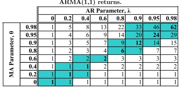
even if we allow returns to deviate from white noise by estimating ARMA(1,1) representations
(which appears to be quite adequate to remove any serial correlation structure in the resulting
residuals) the resulting representations have very low R2s.
Thus the first key (and probably uncontentious) feature that informs our analysis is that
returns are, at best, barely predictable in terms of their own past.
Table 1. Bootstrapped p-values under the white noise null
max(Absolute Autocorrelation) min (p-value on Qtest) min (Variance Ratio)
hmax 1871-2008 1945-2008 1871-2008 1945-2008 1871-2008 1945-2008
10 0.089 0.797 0.095 0.643 0.225 0.648
20 0.196 0.835 0.142 0.762 0.165 0.761
30 0.314 0.967 0.193 0.796 0.032 0.155
40 0.452 0.973 0.262 0.554 0.074 0.030
Notes to Table 1 We simulate the white noise null by resampling with replacement from the empirical distribution of real annual stock returns, in 10,000 repetitions. Thefirst two columns of Table 1 show the bootstrapped probability of a larger value than in the data for the maximum autocorrelation from 1 to hmax, under the white noise null. For Columns 3 and 4, we carry out Ljung-Box Q tests of
the joint significance of autocorrelations from 1 to h, in the data, and in each replication, thenfind the minimum nominal p-value over h=1 to hmax: the table shows the probability, across all replications,
2.2
The variance ratio slopes downwards
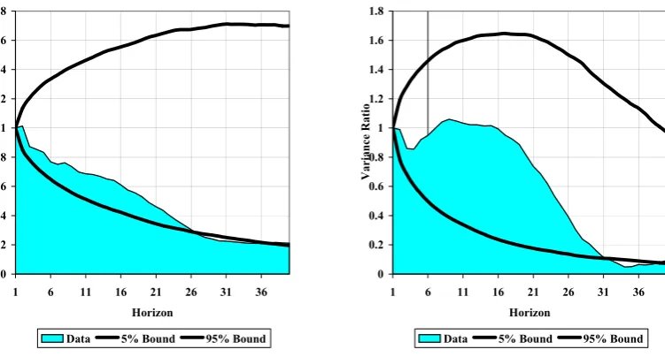
In Figure 2 we show the sample variance ratio for real annual stock returns at horizon h,
[image:9.595.101.477.209.411.2]V R(h) =V ar(Phi=1rt+i)/(V ar(rt).h) for horizons 1 to 40.8
Figure 2. The Variance Ratio of Real US Stock Returns
1871-2008 0 0.2 0.4 0.6 0.8 1 1.2 1.4 1.6 1.8
1 6 11 16 21 26 31 36
Horizon Va ria n ce Ra tio
Data 5% Bound 95% Bound
1945-2008 0 0.2 0.4 0.6 0.8 1 1.2 1.4 1.6 1.8
1 6 11 16 21 26 31 36
Horizon Va ria n ce Ra tio
Data 5% Bound 95% Bound
The first panel shows clearly, over the long sample 1871-2008, the pattern identified by
Poterba & Summers, (1988). The sample variance ratio declines nearly monotonically as the
horizon increases until aroundh= 30,at which point it appears to level out at a value of around
0.2: thus indicating a reduction in volatility for long-horizon returns that is, in economic terms,
highly significant, compared to the white noise benchmark. This pattern has been widely used
to argue that investment in stock portfolios is relatively less risky at long horizons.9 We also
show simulated 5% and 95% bounds for the sample variance ratio under the bootstrapped white
noise null. The observed pattern does not differ much from white noise at short horizons; but
appears increasingly different as the horizon lengthens. While the data mining critique again
8We donot include the small sample adjustment proposed by Cochrane (1988) and others. Given our focus on simulated results, where the variance ratio is calculated in the same way in both data and simulations, any adjustment is unnecessary. Under the white noise null the unadjusted sample variance ratio is biased downwards; however under alternatives where returns are near-white noise such as the ARMA(1,1) we analyse below, we show that the unadjusted sample variance ratio appears to be close to unbiased.
argues against placing too much weight on individual horizons, the third and fourth column of
Table 1 shows that if we focus on the minimum variance ratio across all horizons up to a given
maximum horizon, the longer the horizon, the lower is the probability of observing such a low
value under the white noise null.10
The second panel of Figure 2 shows that if we calculate the variance ratio only over the
postwar period there is no systematic tendency to decline untilh= 20- a result consistent with
the estimates in Kim et al (1991). However, for longer horizons the decline is quite marked,
and, as Table 1 shows, statistically significant against a white noise null, even allowing for the
rather limited number of degrees of freedom.11 We shall show below that there are also clear
indirect measures of a declining variance ratio that persist into the postwar era.
There is no necessary contradiction between our weak rejection of the white noise null for the
autocorrelation function and the stronger results for the variance ratio, since the latter relates
to a long weighted average of autocorrelations.12 In principle “variance compression”13 can be
both quite significant, and consistent with a very limited degree of short-term predictability.
This is indeed what appears to be the case in the data.
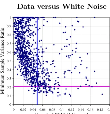
It should also be stressed that the probability that both these features would appear in the
data would be very small under the white noise null. Figure 3 illustrates for the full sample.
We resample 138 observations of the real stock return to simulate the white noise null. Figure
10Pastor & Stambaugh (2008) Figure 10 shows an almost identical pattern using a longer sample, starting in 1802, which implies an even stronger rejection of the white noise null.
11The downward bias noted in footnote 8, which is quite severe in such a relatively short sample, is very evident in the simulated upper and lower bounds.
12From Cochrane’s (1988) orginal analysis showed, we haveV R(h) = 1 + 2hP−1
j=1
³
h−j
h
´
corr(rt, rt−h).
13This feature is often referred to as mean reversion (following Poterba & Summers, (1988)), but we avoid this term deliberately, first, because this usage is not universal (cf Pastor & Stambaugh, 2008); and second, because it is a somewhat confusing misnomer. Poterba & Summers define mean reversion as "stock prices (or cumulative returns) have a mean-reverting transitory component". Following Beveridge & Nelson (1981) we can write any general ARMA(p, q)univariate representation of returns as
rt=a(L)εt=a(1)εt+a∗(L)(1−L)εt
with the second term defining the mean-reverting transitory component in cumulative returns = a∗(L)ε
t.
Such a term will be present forany stationary univariate representation where returns have some serial correla-tion structure, but not all such representacorrela-tions will have a downward sloping variance ratio. It is straightforward to show thata(1)<1is a sufficient condition for the variance ratio to slope downwards. Sincea(1) +a∗(0) = 1,
3 is then a scatter plot of the minimum variance ratio, over horizons 1 to 40, against the sample
R2 for an ARMA(1,1) representation of returns, for each replication. The crossing point of the
[image:11.595.196.377.177.365.2]two lines on the chart shows the values observed in the data.
Figure 3. Univariate Predictability and a Declining Variance Ratio: Data versus White Noise
0 0.1 0.2 0.3 0.4 0.5 0.6 0.7 0.8 0.9 1
0 0.02 0.04 0.06 0.08 0.1 0.12 0.14 0.16 0.18 0.2
Sample ARMA R-Squared
M
inimum Sample Variance R
atio
Figure 3 shows that the bulk of replications would have a low ARMA R2, but with
con-siderable spread: 24% of the sample estimates of the ARMA R2 would be above the value in
the data (very much in line with the evidence on the autocorrelations shown in Table 1). The
majority of simulations would generate a minimum variance ratio well above that in the data;
the points below the horizontal line correspond to the 7.4% probability given in the bottom
row of Table 1. But, most strikingly, samples in which the variance ratio does appear to slope
significantly downwards are almost always also samples in which the ARMA model appears to
predict distinctly better than in the data: only 1.4% of replications generated combinations in
the bottom left quadrant, ie, with both a lower R2 and a lower minimum variance ratio than
in the data.14
3
The predictive regression framework
3.1
The general system
Consider the system used by Stambaugh (1999) and many others in the analysis of predictive
return regressions
rt = −βxxt−1 +ut (1)
xt = λxt−1+vt (2)
where the first equation captures the degree of predictability of some variable rt, typically
stock returns or excess returns over some interval, in terms of a predictor variable xt−1, and
the second describes the autocorrelation of the predictor variable. We assume 0 ≤ λ < 1, so
that bothrt andxt are stationary.15 We put no restrictions on the innovations ut andvt other
than that they be (jointly) serially uncorrelated mean zero withfinite variance. We assume all
data are de-meaned for simplicity, hence neglect constants.
Equation (1) is quite general, since xt−1 may in principle be some weighting of a set of
variables with predictive power forrt and the error term may capture a range of nonlinearities.
Equation (2) is distinctly more restrictive, but, since Stambaugh (1999) has been widely used in
the literature and, again, allowing for exotic errors, can still encompass a wide range of models
(including for example two state Markov switching models, Hamilton 1989).16
Substituting from (2) into (1) we derive the reduced form process for rt, which is an
ARMA(1,1):17
rt=λrt−1+εt−θεt−1 =
µ
1−θL
1−λL ¶
εt (3)
15Most of our results generalise to, but are complicated by,λ <0;however we regard this as empirically less likely to be of interest.
16Apart from differences in notation, our predictive framework is also identical to, eg, Cochrane (2008); Campbell, Lo and Mackinlay (1997), Chapter 7 and Pastor & Stambaugh (2009) (in the the latter context,
xtwould be characterised as a “perfect predictor” -ie, one that captures all available information relevant to
expected returns).
17By letting x be a vector process, with an AR matrix with p distinct roots, we can generalise up to an ARMA(p, p)representation ofrt. We note below that some of our results below still apply in this much more
where L is the lag operator, such thatLxt=xt−1; εt is a serially uncorrelated innovation; and
as long asutandvtare less than perfectly correlated, we can choose the “fundamental” solution
for the MA parameter that hasθ ∈(−1,1), so the representation is strictly invertible in terms
of the history ofrt.18 Ifθ =λ the AR and MA components cancel, andrt will be white noise.
Wefirst note that in the ARMA representation the properties ofrt are entirely determined,
up to a scaling factor, by the pair (λ, θ). The properties of the underlying predictive system
(1) and (2) can in turn be characterised by the three unit-free parameters (λ, ρ, Rx2) where
ρ=σuv/(σuσv)is the Stambaugh Correlation, and R2x = 1−σ2u/σ2r is the R2 in the predictive
regression. We shall refer to the triplet (λ, ρ, R2
x) as the “predictive space”.
The autoregressive coefficient of the predictor variable translates directly to the AR coeffi
-cient of the reduced form (3). For the case of the MA parameterθ things are more complicated.
In Appendix A we show that, subject to an innocuous normalisation on the sign ofβx, θdepends
on all three parameters that define the predictive space,
θ =θ¡λ, ρ, R2x¢ (4)
We shall show that the two univariate properties summarised in Section 2 mean that the
predictive space can be quite tightly constrained. In so doing it will be helpful to make reference
to two important benchmark cases that we shall show determine the nature of these restrictions.
3.2
“Pseudo Predictor” Representations
In this section we define two limiting cases of the predictive system in (1) and (2), both of
which can be derived directly from the properties of the ARMA representation. We shall then
go on to show, in Section 4, that these limiting cases provide benchmarks that allow us to set
limits on the “predictive space” that containsall possible predictive systems of the form in (1)
and (2).
3.2.1 The fundamental pseudo predictor
We can rewrite the ARMA(1,1) representation in (3) as a predictive system of the same general
form as (1) and (2):19
rt = −βfxft−1+εt (5)
xft = λx f
t−1+εt (6)
where βf = θ − λ, and we refer to the predictor variable, xft, as the “fundamental pseudo
predictor”. It has the same AR(1) form as the true predictor variable, but with innovations
identical to those in the predictive regression, hence the Stambaugh Correlation is precisely
unity. It will generate identical predictions to the fundamental ARMA representation in (3),
and will therefore have the same predictive R2, which we show in Appendix B is given by
R2f(λ, θ)≡1− σ
2
ε σ2
r
= (θ−λ)
2
1−λ2+ (θ−λ)2 (7)
Note that, using (6) and (3) we can also write
xft = rt 1−θL =
∞ X
i=0
θirt−i (8)
so the fundamental pseudo predictor is simply an exponentially weighted moving average of
rt.20
19See Appendix A.
20An alternative interpretation of xf
t is, up to a scaling factor, as the optimal estimate of the true
predic-tor xt given the information set {ri}ti=−∞. Cochrane (2008b) refers to this as the “Observable State Space
3.2.2 The non-fundamental pseudo predictor
For every fundamental ARMA(1,1) representation with θ 6= 021 there is an associated
“non-fundamental” representation, given by
rt=
µ
1−θ−1L
1−λL ¶
ηt (9)
withσ2
η =θ
2
σ2
ε.This representation generates an identical autocorrelation structure for returns
to that of the fundamental representation, but, as is well known (see for example Hamilton,
1994, pp 66-67), the non-fundamental innovations, ηt cannot be recovered from the history of
rt, hence the non-fundamental representation does not represent a viable predictive model. As
a result, with a few exceptions (Lippi & Reichlin 1994; Hansen & Sargent, 2005;
Fernandez-Villaverde, Rubio-Ramirez, Sargent, and Watson, 2007) non-fundamental representations have
received relatively little attention.
To see why ηt cannot be recovered from the data, note that if we attempt to solve (9) for
ηt we have
ηt = µ
1−λL
1−θ−1L ¶
rt =
∞ X
i=0
θ−i[rt−i−λrt−i−1]
given that¯¯θ−1¯¯>1the sum does not converge, hence the representation in (9) is not invertible
in terms of the history of rt. However, if (strictly hypothetically) we had data on current and
future values ofrt, we could write
ηt =
µ
1−λL
1−θ−1L ¶
rt =−θF µ
1−λL
1−θF ¶
rt=−θ ∞ X
i=1
θi[rt+i−λrt+i−1] (10)
where F is the forward shift operator, such that F xt = L−1xt = xt
+1, and in this case the
sum does converge. Thus the non-fundamental ARMA representation does have an invertible
representation, but only in terms of current and future values of rt, making it valueless as a
predictive model.
Of course, if we already knew the entire future of rt, we would not need a predictive model
at all, therefore there would be no point in constructing a series for ηt. But the reverse is not
the case. In general, even if we did have data onηt (perhaps by some divine dispensation) this
would not reveal the entire future of rt, but rather a particular linear combination of future
values. Thus while (as we show below) the non-fundamental representation would, if we had the
history ofηt,predict better than the fundamental representation, it would not predict perfectly.
While it may seem somewhat peculiar to take an interest in a predictive model that is so
manifestly non-viable, it turns out that it provides us with an extremely useful benchmark.
And it does so because, while we will never be able to observe ηt in practice, we do know
the predictive properties of the non-fundamental representation, even if we cannot actually
use it to predict, since these can be inferred directly from the properties of the fundamental
representation.22
As noted above, the equivalence of the two representations must imply that, for θ 6= ±1,
ηt has lower variance than εt, the fundamental innovation (since σ2η =θ
2
σ2
ε), hence, if we did
have data on ηt, the non-fundamental representation would predict strictly better than the
fundamental representation. Its (strictly notional) predictiveR2 can be derived by replacingθ
with θ−1 in (7), giving
R2n(λ, θ)≡1− θ
2
σ2
ε σ2
r
= (1−θλ)
2
1−λ2+ (θ−λ)2 > R
2
f(λ, θ) ; for θ∈ (−1.1) (11)
As for the fundamental ARMA representation, we can again reverse-engineer a
representa-tion of the same general form as (1) and (2), and write
rt = −βnxnt−1+ηt (12)
xnt = λxnt−1+ηt (13)
22In Lippi & Reichlin’s (1994) terminology the fundamental representation in (9) is a “basic”
non-fundamental representation, in that it is of the same order as the observable non-fundamental representation. There is in principle an infinity of "non-basic" non-fundamental representations of arbitrary higher order, since any white noise innovation can always be given a non-fundamental representation: ie, we could write
ηt=
¡
1−φ−1L¢(1−φL)−1ωt, withσ2ω =φ2σ2η, and in principle then find a non-fundamental representation
of ωt,and so on ad infinitum. But nothing in the data tells us anything about φ, and hence about ωt,hence
withβn =θ−1−λ, wherexn
t,the “non-fundamental pseudo predictor” has the same innovations,
and the same predictive R2 for rt, as the non-fundamental ARMA representation, and again
has a Stambaugh Correlation of precisely unity.
3.3
The variance ratio in the ARMA(1,1) reduced form
We have already referred, in our discussion of univariate properties in the data, to the variance
ratio at horizon h, as originally defined for the general case by Cochrane (1988) as
V R(h) = 1
h
V ar(Phi=1rt+i)
V ar(rt) (14)
It is straightforward to show23 that, for the ARMA(1,1) process (3), V R(h) is monotonic inh
and that
V R(h)
⎧ ⎪ ⎨ ⎪ ⎩
<1⇔θ > λ
>1⇔θ < λ
;∀ h >1 (15)
We shall also make use of the limiting value of the variance ratio, which in the ARMA(1,1) can
be expressed as
V = lim
h→∞V R(h) = (1−R
2
f) µ
1−θ
1−λ ¶2
(16)
where, given the monotonicity of theV R(h) inh, we also haveV <1⇔V R(h)<1∀h >1.
4
The Predictive Space for Stock Returns
4.1
Bounds on the ARMA(1,1) coe
ffi
cients,
θ
and
λ
In Section 2 we discussed two univariate properties of real stock returns in the data: first that
they were near-white noise (hence barely predictable in the short term); and second that there
appears to be quite strong evidence of “variance compression” (ie, a declining variance ratio).
It is straightforward to show that these two features of the data constrain quite tightly the
possible values ofλ andθ in the ARMA representation. We shall subsequently see that this in
turn will place quite significant restrictions on the predictive space.
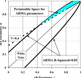
Using the ARMA(1,1) framework outlined above we show, in Figure 4, contours in (θ, λ)
space of equal R2
f and of equalV (the limiting value of the variance ratio).24 The top panel of
Figure 4 shows contours forV = 0.4andR2
f = 0.05. The shaded area then gives the admissible
set of (θ, λ)that generate values ofV no greater than 0.4 and R2
f of no more than 0.05. Lower
values of V push the V-contour up and to the left, while lower values of R2
f move the R2f
-contours towards the 45 degree line, thus reducing the admissible(θ, λ)area. The second panel
of Figure 4 illustrates: the shaded area is now the (θ, λ) combinations consistent with V no
greater than 0.2, and R2
f below 0.025: the permissible space for both ARMA parameters now
becomes very tightly constrained: λ must be quite close to unity, and θ must be even closer.25
We showed in Section 3 that the ARMA representation inherits the AR parameter λ from
the true predictor. Figure 4 shows that the requirement that λ be large arises naturally from
the univariate properties of returns. Virtually all observable predictors of stock prices (most
notably valuation ratios like the price-dividend ratio or the price-earnings ratio) have this
characteristic.26 But the analysis illustrated by Figure 4 shows that, for sufficiently strong
variance compression, and sufficiently weak short-term univariate predictability, the same must
apply for any logically possible predictor.
We now go on to show that these univariate features can put significant restrictions on the
predictive space of the underlying model that generates them.
24For given values ofR2
f andV,we solve (7) and (16) forθin terms ofλ. The former gives two solutions for
θ,symmetric around the 45 degree line. 25The numbers used for R2
f and V in Figure 4 are illustrative, but are quite consistent with the evidence
illustrated in Figures 1 to 3. Sample estimates ofR2
f are, ifλis high, subject to severe Stambaugh (1999) bias.
Simulation evidence shows that even in a sample as long as the 1871-2008 period discussed in Section 2 a true
R2
f of 0.025 would result in a mean sample estimate at least twice as large, thus consistent with what we observe
in the data. For large λand θ we can also haveV R(h)well above the limiting value V even for horizons as long as those shown in Figure 2.
Figure 4
The Permissible Space for ARMA Parameters for Stock Returns
0 0.2 0.4 0.6 0.8 1
0 0.2 0.4 0.6 0.8 1
AR Parameter, λ
M
A
Param
et
er,
θ
V=0.4
ARMA R-Squared=0.05 Permissible Space for
ARMA parameters
White Noise
Limiting variance ratio, V≤0.4; ARMA R-Squared ≤ 0.05
0 0.2 0.4 0.6 0.8 1
0 0.2 0.4 0.6 0.8 1
AR Parameter, λ
M
A
Param
et
er,
θ
V =0.2
ARMA R-Squared=0.025 Permissible Space for
ARMA parameters
White Noise
4.2
Bounds for the one-period-ahead predictive
R
2Proposition 1 For a fundamental ARMA(1,1) representation of returns which is a reduced
form of a predictive regression (1) and a predictor autoregression (2) the one-period-ahead R2
of the predictive regression, R2x, satisfies
R2f(λ, θ)≤Rx2 ≤R2n(λ, θ) (17)
where R2
f and R2n are as defined in (7) and (11).
Proof. See Appendix D. The lower bound for R2
x is the predictive R2 of the fundamental ARMA representation,
or, equivalently, of the “fundamental pseudo predictor” defined in Section 3.2.1. As such it is
quite easy to interpret. As long as the true predictor provides some predictive information for
rt beyond that contained in the history of rt itself (ie, if βx 6= 0, ρ ∈ (−1,1)) it must have a
strictly higher predictive R2; only if β
x = 0, or in the special case of the fundamental pseudo
predictor, is the lower bound attained.27
The upper bound forR2
x is the predictiveR2 of thenon-fundamental ARMA representation,
or equivalently of its associated pseudo predictor, defined in Section 3.2.2. The intuition for
this result can be related to our earlier discussion of the properties of the non-fundamental
representation. We showed in Section 3.2.2 that the non-fundamental innovation ηt can be
expressed, in (10), as a linear combination of current and future returns: so we know already
that it must have some predictive power beyond that already in the history of returns. But
the result in Proposition 1 is distinctly stronger: it shows that the non-fundamental pseudo
predictor in periodtis the bestpossiblepredictor ofrt+1consistent with its observable univariate
properties.28
27We noted in Section 3.2.1, the alternative interpretation of the fundamental pseudo predictor, xf t as the
optimal estimate of the true predictor xt given the information set {ri}ti=−∞. If we have data on xt, rather
than its estimate, we must be able to predict better, except in the special case thatxt=xft.
28Given the ARMA(1,1) property of returns we know that the true predictor must be an AR(1). For
We shall show that when the ARMA parameters, θ andλ, lie within the permissible range
illustrated in Figure 4, for a given degree of variance compression and low short-term
pre-dictibability then the allowable range of R2
x given by Proposition 1 can become quite small.
We have already noted that if θ =λ returns are white noise. This arises trivially if βx = 0.
But there is also a more interesting special case:
Remark (Predictable White Noise) If R2
x > 0 but θ(λ, ρ, R2x) = λ, the inequality in
(17) reduces to
0< Rx2 ≤1−λ
2
We discuss the properties of this special case in more detail in Section 4.5 below.
4.3
Bounds for
ρ
for predictor variables
Our focus thus far has been on just two of the elements in the predictive space, namelyλ and
R2
x. But a further important feature of Proposition 1 is that both the upper and lower bounds
arise in limiting cases of the predictive system (in (5) and (6), and in (12) and (13)) for which
the Stambaugh Correlation,ρ, is precisely unity. We now examine intermediate cases in which
the innovations are not perfectly correlated.
We have from (4) that the ARMA coefficientsθ andλare linked to the predictiveR2
xand the
Stambaugh Correlation between the innovations, ρ,by θ=θ(λ, ρ, R2
x).Thus for a given(θ, λ)
pair there is a contour of possible values of (R2
x, ρ) consistent with the ARMA representation.
Again it turns out that the univariate properties of rtimpose limits on the possible values ofρ.
Proposition 2 Consider a fundamental ARMA(1,1) univariate representation (3) which is a
reduced form of a predictive regression (1) and a predictor autoregression (2). For0< λ < θ(ie
the variance ratio slopes downwards and the predictor has positive persistence) the Stambaugh
correlation ρ satisfies
|ρ|≥ρmin(λ, θ)>0
Proof. See Appendix E.
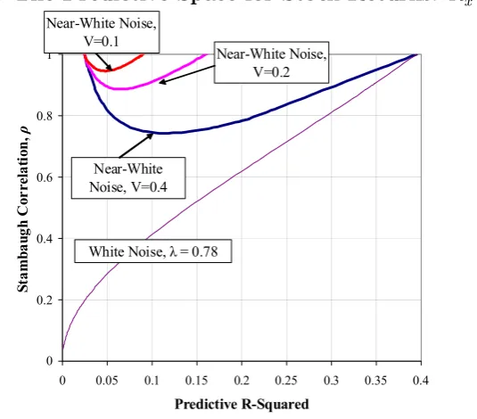
Figure 5 illustrates the link betweeen Propositions 1 and 2. We graph the contours in(R2x, ρ)
we constrain ρ to be non-negative (which we can always ensure is the case by an appropriate
[image:22.595.172.440.143.378.2]rescaling of the data forxt).29
Figure 5. The Predictive Space for Stock Returns: R2
x and ρ
0 0.2 0.4 0.6 0.8 1
0 0.05 0.1 0.15 0.2 0.25 0.3 0.35 0.4
Predictive R-Squared
St
am
ba
ug
h
C
or
re
la
ti
on
,
ρ
White Noise, λ = 0.78 Near-White Noise, V=0.4
Near-White Noise, V=0.2 Near-White Noise,
V=0.1
Figure 6. The correlation between the true predictor and the fundamental pseudo predictor
0 0.2 0.4 0.6 0.8 1
0 0.05 0.1 0.15 0.2 0.25 0.3 0.35 0.4
Predictive R-Squared
corr(
x,
xf
)
Lower Bound, Near-White Noise, V=0.4
Lower Bound, Near-White Noise, V=0.2 Lower Bound, Near-White Noise, V=0.2
As a benchmark for comparison, the lowest contour line shows combinations of the two
parameters consistent with the special case of predictable white noise noted in the previous
29As noted in the introduction,ρwill be positive ifx
tis expressed as a log ratio of price to fundamental, and
[image:22.595.182.414.452.651.2]section, when the predictor is quite strongly persistent (θ =λ = 0.78).The better the predictive
model, the higher the associated Stambaugh Correlation, ρ, must be. While ρ can take any
value in[0,1], the lower bound forρ will only be attained withR2
x = 0. Thus even in the white
noise case anyuseful predictor with positive λ must also have non-zeroρ.
The remaining contour lines represent a range of near-white noise processes, all with the
same univariate R2 (R2
f = 0.025) but with progressively stronger degrees of variance
compres-sion (ie, lower values ofV). For a given degree of short-term predictability, this correponds to a
progressive reduction in the upper bound forR2x.Sinceρ = 1at both upper and lower bounds,
the range of possible values of ρ is progressively reduced, henceρmin in Proposition 2 becomes
progressively closer to unity.This feature of our results sheds light on a significant feature of
the the empirical literature on predictive regressions. In most of this literature a high value of
the Stambaugh Correlation is usually treated simply as a nuisance that complicates inference.
Our results show that when returns have declining variance ratios (or even if they are purely
white noise) it is an intrinsic feature of the true predictor of returns.30
4.4
How di
ff
erent are predictor variables from the history of
re-turns?
We have shown in the previous section that, given observable univariate properties of returns,
the Stambaugh Correlation is likely to be close to unity in absolute value (ie, innovations to the
predictor variable will be strongly correlated with innovations in the predictive regression). We
also know that, by construction, the fundamental pseudo predictor, which from (8) is simply
a weighted average of past returns, has a Stambaugh Correlation of precisely unity. It might
therefore seem that any predictor must resemble the pseudo predictor quite closely. In fact,
while this may be the case for certain univariate processes, the correlation between the true
predictor and the fundamental pseudo predictor can in principle cover a distinctly wider range
than the Stambaugh Correlation, as the following proposition shows:
Proposition 3 If xt is the true predictor in the predictive regression (1), with predictive
R-squared R2
x, and x f
t is the fundamental pseudo predictor, which, from (8) can be constructed
from the history of returns, then
corr(xt, xft)2 = R2
f R2
x
≥ R
2
f R2
n
= 1
θ2 µ
θ−λ θ−1−λ
¶2
where R2
f(λ, θ) and R2n(λ, θ) are the upper and lower bounds given in Proposition 1.
Proof. See Appendix F.
By inspection of the relationship in Proposition 3, it is evident that in the limiting case of
white noise returns (θ = λ) the correlation is precisely zero, since R2
f = 0. Indeed it is of the
essence of a white noise process that it its own history is entirely uninformative about its own
future values, and hence it must be uninformative about any predictor of its future values.
For near-white noise processes the correlation is non-zero, and the proposition shows that
the better the true predictor predicts, the less similar it will be to the fundamental pseudo
predictor. But the upper bound on R2x given in Proposition 1 implies a lower bound on the
correlation in Proposition 3: hence the narrower is the range of possible values of R2
x,the more
similar the true predictor must be to the fundamental pseudo predictor. The lower bound
in Proposition 3 is determined by the relative predictive power of the fundamental vs
non-fundamental representations.
Figure 6 (below Figure 5) illustrates, for the three near-white noise processes already
illus-trated in Figure 5. Since all three have the same value ofR2
f,the univariateR2, the relationship
between corr³xt, xft ´
and R2x given in Proposition 3 is identical for all three processes. If the
true predictor predicts barely any better than the univariate representation, it will very closely
resemble it, but the better it predicts the weaker this resemblance will be. The only impact
of greater variance compression (a lower value of V) will be that, since this reduces the upper
bound for R2
x, it must increase the lower bound for corr ³
xt, xft ´
(the lower bounds for each of
the three processes are shown as dotted lines).31
However, Figure 6 illustrates that even when there is very significant variance compression
(as θ approaches unity) there is still scope for the true predictor to look quite dissimilar to
the fundamental pseudo predictor. This suggests a simple pre-test when looking for predictor
variables for stock returns: we should seek those that do not simply look like the history of
returns.
4.5
A special case: predictable white noise
We have already noted, in our discussion of Proposition 1, that the special case in which returns
are entirely unpredictable from their own past does not rule out predictability from some other
predictor variable. This case is worth considering not just as a benchmark for comparison,
but also because it is an implication (whether implicit or explicit) of a range of revisionist
investigations of return predictability. Some of these (eg, Goyal & Welch, 2003) have concluded
that there is simply no return predictability at all of any kind (ie, βx = 0) ; others (eg Kim et
al, 1991) have concluded that the true variance ratio does not differ significantly from unity at
any horizon, which must imply directly that there may be little or no univariate predictability
(ie, the more general white noise case θ =λ). Even defenders of return predictability such as
Campbell & Viceira (2002), Cochrane (2005, Chapter 20) have acknowledged the possibility
that there may be no univariate predictability.
Of course if returns are white noise, we have no way of inferring anything directly from
the history of returns about the values of the ARMA parameters, except that they must be
equal. But this still tells us something about the predictive space: that it depends on a
single parameter, λ,the persistence of the true predictor, since the white noise property means
that the predictive space must always satisfy θ(λ, ρ, R2
x) = λ. We noted in Section 4.1 that
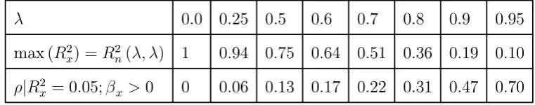
most observable predictors of stock returns are strongly persistent. In Table 2 we show that
the maximum possible predictive R2, as given by Proposition 1, declines as λ increases. For
strongly persistent predictors the scope for return predictability, from any possible predictor
Table 2. The predictive space if stock returns are white noise
λ 0.0 0.25 0.5 0.6 0.7 0.8 0.9 0.95
max (R2x) =R2n(λ, λ) 1 0.94 0.75 0.64 0.51 0.36 0.19 0.10
ρ|R2
x = 0.05;βx >0 0 0.06 0.13 0.17 0.22 0.31 0.47 0.70
Notes to Table 2 In line 1 of the Table we show the maximum predictive R2 for a white noise
process, using Proposition 1, which implies max (R2
x) = 1−λ
2
. Line 2 shows the required value of the Stambaugh correlationρ, for a given value ofR2x using equation (39) settingθ =λ. We constrain ρ to lie in[0,1]by normalisation of the data for xtsuch that βx >0 .
At the other extreme, Table 2 also highlights a further special case of a white noise predictor
of white noise returns (ie, λ = θ = 0). This is the sole case for which the inequality in
Proposition 1 is devoid of content, since it reduces to the condition thatR2x ∈[0,1].In this case
the predictor has (trivially) the same ARMA order as returns (ie, they are both ARMA(0,0)),
which therefore nests the case: xt = rt+1 ⇒ R2x = 1. Thus in this case the absolute upper
bound for R2
x can be attained, at least in logic, if not (in the absence of divine dispensation or
time travel) in practice.32
As noted in our discussion of Proposition 2, the predictable white noise case means that,
subject to our normalisation ofxt,the Stambaugh Correlation,ρ,can in principle live anywhere
in[0,1] ;but auseful predictor withλ, βx >0must have a positive Stambaugh Correlation, and
the better it predicts the higherρmust be (since the limiting case of the best possible predictor
is the non-fundamental pseudo predictor defined in Section 3.2.2, with ρ = 1). Furthermore,
for any given value ofR2
x, ρ is also increasing inλ, because a higher value ofλbrings down the
upper bound at which ρ equals unity. The bottom row of Table 2 illustrates this relationship.
This necessary link betweenρ, R2
x andλin the case of predictable white noise returns casts
another interesting light on the predictability literature. As noted above, valuation ratios such
as the price-dividends and price-earnings ratios have frequently been proposed as predictors of
returns. In Robertson & Wright (2009) we show that a range of such predictors all have AR(1)
parameters in the neighbourhood of 0.9; with estimated Stambaugh Correlations also around
this value, or in some cases, even closer to unity. In contrast the bottom row of Table 2 shows
32Note that the key condition here is actuallyθ= 0,which, from (37), always impliesmax¡R2 x
¢
=R2
that for white noise returns, and R2
x = 0.05 (a figure not out of line with those found in the
return predictability literature) the required value ofρforλ = 0.9is very much lower than this.
An immediate conclusion that follows is that it would not be possible to claim simultaneously
that any one of these predictors is the true predictor, and that returns are white noise. We
shall see in the next section that higher values of ρ are more consistent with a predictor of
a return process with a declining variance ratio, but in that case the univariate predictability
that necessarily follows from this provides an alternative benchmark against which to compare
such predictors. In Robertson & Wright (2009) we conclude that none of these commonly
used predictors can be distinguished in the data from the pseudo predictor consistent with this
univariate predictability.
5
The predictive space for real US stock returns
1871-2008: some empirical estimates
In estimating the limits to the predictive space consistent with the observed history of returns
examined at the start of the paper, we should note at the outset that, given the near-white noise
properties of returns, no method of estimation can be expected to yield well-determined results.
Nor do we wish to pin ourselves down to any assumption that the univariate representation has
been stable, and of the restrictive ARMA(1,1) form, over the entire sample of returns.33 Our
estimates in this section are thus largely illustrative.
Even in the absence of any empirical estimates, it should be noted that, simply by allowing
for the possibility that returns may be near-white noise with a declining variance ratio, it follows
straightforwardly that, for any given degree of predictor persistence, the predictive space must
contract relative to the white noise case. Variance compression requiresθ > λ. This raises R2
f,
the fit of the fundamental ARMA representation, above zero, but at the same time decreases
33It is quite possible that there may have been structural shifts in the ARMA parameters as well as both
the maximum possible predictive R2 (that of the non-fundamental representation, R2
n.) thus
contracting the space thatR2
x can feasibly inhabit. At the same time, from Propositions 2 and
3, increasing variance compression raises towards unity the lower bounds on both the absolute
Stambaugh Correlation and the correlation between the predictor and the fundamental pseudo
predictor. Thus on the basis of a priori reasoning alone we know that greater is the degree of
variance compression, the more the predictive space must contract.
Our starting point is simply to estimate the ARMA representation. There are obvious
caveats: the near-white noise property means that the AR and MA components are very close
to cancellation, and thus, as is well known, bothλ andθ are likely to be poorly estimated, and
subject to significant small-sample (essentially Stambaugh, 1999) bias. There is however an
important cross-check on our results, in the spirit of Cochrane, 1988. We showed in Section 3.3
that in the ARMA(1,1) there is a direct correspondence between the sign ofθ−λ and the slope
of the variance ratio. It is also straightforward to show34 that, ifθ > λ, therate at which the
variance ratio slopes downwards is determined solely by the magnitude ofV (λ, θ)(the limiting
variance ratio) and λ. In principle direct measurement of the variance ratio could, for some
processes, yield very different answers from that implied by ARMA estimates;35 but in both
the long annual sample 1871-2008 and (with caveats) the shorter postwar sample 1945-2008,
the results are reassuringly similar.
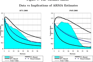
Figure 7 illustrates. We estimate ARMA(1,1) representations of returns in both samples.
In terms of the expectations derived from our analysis thus far the point estimates are certainly
in the right ballpark: for the full sample we havebλ = 0.860 andbθ = 0.977, and in the postwar
sample we have bλ = 0.89 bθ = 0.95, thus in both samples the point estimates are consistent
with variance compression,36 but they are somewhat closer together in the postwar sample,
and hence returns are somewhat closer to white noise. Figure 7 shows that if we treat the
ARMA estimates as equal to their true population values, the results are not in conflict with
the evidence from direct measurement of the variance ratio.
34See Appendix C.
35See, for example, the comparison between the very different implications of the variance ratio and ARMA representations of GNP growth in Cochrane, 1988.
Figure 7. The Variance Ratio:
Data vs Implications of ARMA Estimates
1871-2008 0 0.2 0.4 0.6 0.8 1 1.2
1 6 11 16 21 26 31 36
Horizon Va ri an ce R at io
Data 5% Bound
95% Bound Mean Estimate `True' Value 1945-2008 0 0.2 0.4 0.6 0.8 1 1.2 1.4
1 6 11 16 21 26 31 36
Horizon Va ri an ce R at io
Data 5% Bound
95% Bound Mean Estimate `True' Value
Notes to Figure 7 We show the variance ratio in the data, as in Figure 2. The 5% and 95% bounds and mean estimates are simulated in 10,000 replications using the estimated ARMA model as the data generating process. The two panels also show the calculated true value of the variance ratio, as given by (34) in Appendix C, on the same assumptions.otes to Table 1. We simulate the white noise null by resampling with replacement from the empirical distribution of real annual stock returns, in 10,000 repetitions.
In the full sample this consistency is particularly marked. The implied “true” horizon
variance ratio matches the sample variance ratio well, particularly at longer investor horizons;
and even when the two profiles differ somewhat at shorter horizons, the deviation is well within
the range of sampling variation.37
In the post-war sample, while the ARMA estimates are quite similar to those estimated
over the full sample, they are less consistent with direct measurement of the variance ratio.
But the differences are not in general statistically significant. Given the short sample, if the
estimated ARMA parameters were truly generating the returns data, the range of sampling
variation of the variance ratio would be quite wide, especially at short horizons, hence the lack
of any decline for horizons up to around 15 years (as noted by Kim et al, 1991) would not of
itself be particularly significant. Indeed the only statistically significant contrast between the
two approaches is at very long horizons, when the observed variance ratio actually breaches the
lower 5% bound consistent with the ARMA estimates being the true model. However, given
the range of uncertainty in both approaches, it is fairly obvious that it would take only a very
limited amount of data mining tofind an ARMA representation that was consistent both with
the direct ARMA estimates and the evidence of the variance ratio, over both samples. Any
such representation would have a high value of λ, andθ > λ.
Given the mutual consistency of the two approaches (particularly in the long sample) we
have no obvious reason, in terms of the variance ratio evidence at least, to object to the ARMA
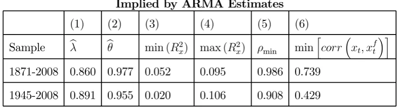
estimates. In Table 3 we therefore take these estimates at face value, and use them to calculate
the implied constraints on the predictive space, using estimates from both long and short
samples.38
The implied value of R2
f the univariate R2, which, from Proposition 1, provides the lower
bound for the predictive R2 of the true predictor is around 5% in the long sample. This
is reasonably consistent with the sample estimate (if anything, given the known impact of
Stambaugh Bias, we might expect the sample value to be rather higher). In the postwar
sample, as noted above, returns appear closer to white noise, hence the implied true R2
f is
distinctly closer to zero.39
For the upper bound, max (R2
x) = R2n, the notional R2 of the non-fundamental ARMA
representation, we have, of course, no cross-check from the data, but we can calculate it directly
from the estimated values of λandθ if we treat them as the true parameters. This calculation
implies that, in both samples, the best possible predictor of stock returns would have an R2 of
around 10%: thus in terms of predictive R2 the predictive space is quite narrow. The implied
space for the Stambaugh Correlation is even more tightly constrained: the point estimate of
ρmin, as defined in Proposition 2, is very close to unity, particularly for full sample estimates.
38We do not report standard errors, because in this region of the parameter space they are likely to be highly misleading.
39Note that in our theoretical analysis we focussed on the true R2,which is a function of the true values of
Table 3 Point Estimates of Limits on the Predictive Space for US Stock Returns Implied by ARMA Estimates
(1) (2) (3) (4) (5) (6)
Sample bλ bθ min (R2
x) max (R2x) ρmin min
h
corr³xt, xft´i
1871-2008 0.860 0.977 0.052 0.095 0.986 0.739
1945-2008 0.891 0.955 0.020 0.106 0.908 0.429
Notes to Table 3Columns (1) and (2) show the estimated autoregressive (λ)and moving average (θ) parameters in estimated ARMA(1,1) representations of returns over the given samples. Columns (3) and (4) give the implied upper and lower bounds for the predictive R-squared from Proposition 1,
given by (column 3)min (R2
x) =R2f ³
b
λ,bθ´and (column 4) max(R2
x) =R2n ³
b
λ,bθ´.Column (5) gives
the implied lower bound,ρmin³bλ,bθ´for the Stambaugh Correlation from Proposition 2. Column (6) gives the lower bound for the correlation between the true predictor and the pseudo predictor, as given
by Proposition 3, as
³ R2
f ³
b
λ,bθ´/R2
n ³
b λ,bθ´´
1/2
.
In the final column of the table we calculate the implied lower bound for the correlation
between the true predictor and the fundamental pseudo predictor. It is noticeable that, despite
the apparently very limited predictive space forR2x andρ,the true predictor can still in
princi-ple look reasonably different from the pseudo predictor - particularly so if we use the postwar
ARMA estimates.40 Nonetheless the clear implication of Table 3 is that point estimates
consis-tent with the data suggest only very little space for any predictor to out-predict the univariate
representation.
Of course, given the known problems in estimating ARMA representations with
near-cancellation of AR and MA roots, the figures in Table 3 should only be treated as illustrative.
We certainly would not wish to state categorically that the true predictive space must be as
narrow as the ARMA estimates suggest. Given sampling variation, the history of returns is
in principle consistent with a range of true data generating processes, some of which have a
distinctly less constrained predictive space. However, if we wish to argue that the predictive
space is less constrained, we show in the next section that this has important implications for
40This reflects the fact that, while the difference betweenR2
f andR2n is small, it is theratio that determines
the lower bound for the correlation, and in the postwar sample in particular this ratio is quite high, despite the low value ofR2
another aspect of return predictability on which we have not yet touched: namely long-horizon
predictability.
6
The predictive space and long-horizon return
predictabil-ity
We have stressed already that the estimates in Table 3 are only illustrative. Given the range of
sampling variation of ARMA estimates we might quite easily derive point estimates of a similar
order of magnitude to those in Table 3 for a quite wide range of white and near-white noise
processes, albeit subject to the following considerations:
• First, and fairly obviously, the true process cannot be very far from white noise. In terms
of Figure 4, the true values of θ and λ must lie within the quite narrow range given by
theR2 contour lines. Hence we would reject any data generating process for returns for
whichθ was very far fromλ.
• Additionally we have strong grounds to reject near-white noise processes with variance
expansion rather than compression (ie, withθ < λ,and hence an upward sloping variance
ratio), given the quite strong rejection of the white noise null by sample variance ratio
data, discussed in Section 2. Even if the true variance ratio had only a modest upward
slope, the probability of observing the low values observed in the data rapidly wouuld be
vanishingly small.
• On the other hand we know that the rejection of the strict white noise case is at best only
marginal. Hence the data also do not reject values ofθ andλ for which the variance ratio
only slopes down very modestly (ie, for whichV is less than, but quite close to unity)
While these considerations rule out quite a wide range of (λ, θ) combinations, it is evident
that the data do admit representations that lie roughly between the 45◦ line and the upper
R2 contour in Figure 4. Since this includes representations in which λ and θ are both close