MULTI CROSS PROTOCOL WITH HYBRID TOPOGRAPHY CONTROL FOR MANETS

ISSN: 1992-8645 www.jatit.org E-ISSN: 1817-3195

711

HIGHLY NONLINEAR RIGID FLEXIBLE MANIPULATOR

STATE ESTIMATION USING THE EXTENDED AND THE

UNSCENTED KALMAN FILTERS

1

MOHAMMED BAKHTI, 2 BADR BOUOULID IDRISSI

1,2

Moulay Ismail University, Ecole Nationale Supérieure d’Arts et Métiers,

BP 4024, Marjane II, Beni Hamed, 50000, Meknes, Morocco.

E-mail: 1 [email protected], 2 [email protected]

ABSTRACT

This paper focuses on the highly nonlinear rigid-flexible manipulator state estimation using the Extended Kalman Filter and the Unscented Kalman Filter. The Hamilton’s principle is used to derive the manipulator equations, the Euler-Bernoulli assumption is considered to model the flexible link, and the elastic movement is approximated using the assumed modes method. The simulation study compares the efficiency of the state estimation quantified by the estimation mean squared error and the time required by the filters to converge.

Keywords: Extended Kalman Filter, Rigid-Flexible Manipulator, Nonlinear Filtering, State Estimation,

Unscented Kalman Filter.

1. INTRODUCTION

Rigid-flexible manipulators are a promising alternative to rigid-rigid ones due to their greater payload to manipulator weight ratio, higher operation speed, larger work space, lower energy consumption and safer operability. However, they exhibit disadvantages of deflection associated with structural flexibility and vibration problem [1]. Their modeling approaches and their control/observation strategies must consider both the rigid body and the flexible degrees of freedom [2].

The Hamilton’s principle is one of the most used approaches when modeling the flexible manipulators. The deformation model of the flexible links is usually based on the Euler – Bernoulli beam theory, and the elastic degrees of freedom are approximated using either the assumed mode method or the finite element method. In general, only first few vibration modes play a significant role in the dynamic equations formulation. As actuators, usually DC motors are used at the manipulator joints due to their simple control scheme.

Most of the active vibration control strategies require the state feedback, and many nonlinear

observer formulations have been addressed for the flexible manipulators. To estimate the elastic degrees of freedom and their time derivatives, a nonlinear high gain observer has been developed by [3], and the sliding mode theory has been investigated by [4] to design both a controller and an observer for the tip positioning problem. Distributed observers have been presented by [5, 6] to estimate infinite dimensional states requiring only the boundary values measured by sensors. An extended state observer was proposed for the trajectory tracking control of a flexible-joint robotic system by [7], and the Extended Kalman Filter has been used by [8] to give an estimate of the environmental forces.

ISSN: 1992-8645 www.jatit.org E-ISSN: 1817-3195

712 sufficiently describing the state pdf [11]. Unfortunately, the EKF requires the nonlinear prediction and measurement function jacobians to be evaluated repeatedly at each time step [12], and this may cause the results to be unreliable and the implementation to be difficult.

A diversion from evaluating the jacobians is allowed by the Unscented Kalman Filter (UKF) [13]. As an alternative, a small set of points, called the sigma-points, are carefully chosen to capture the mean and covariance of the state before they undergo the system nonlinearities. Once transformed, those points are used to evaluate the mean and covariance of the state to be estimated. Contrarily to the Monte Carlo method, the samples are not drawn at random, yet they are deterministically selected so that they capture the essential information about the state pdf.

Preceding research paper addressed the nonlinear optimal state estimation under parametrice uncertianties based on the EKF and the UKF for a one-link flexible manipulator [14,15]. Based on simplifying assumptions, a linear model of the flexible manipulator was targetted by a Model Predictive Control scheme associated to a state estimation based on Kalman filter in [16].

The main contribution of this paper is to compare the EKF and the UKF algorithms when used to estimate the state of a highly nonlinear 2 Degrees of Freedom (2DOF) rigid-flexible manipulator. The analyzed motion of the manipulator is fully described by the rigid body motion, and the vibration motion. Thus the state vector consists of the shoulder joint angle, the elbow joint angle, the first modal coordinate and their respective time derivatives. The flexible link deformation is described using the Euler-Bernoulli theory, the elastic degree of freedom is approximated using the assumed mode method, and the system equations are derived using Hamilton’s principle.

In the next section, the mathematical model for the rigid-flexible manipulator is derived, while in section 3, the EKF and the UKF principles and algorithms are detailed. Simulation results are displayed and discussed in section 4, and conclusion are outlined in section 5.

2. MATHEMATICAL MODELING OF THE

RIGID-FLEXIBLE MANIPULATOR

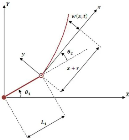
The shoulder and elbow joint angular positions, driven by servo motors, are respectively θ and θ , and L denotes the length of the rigid link. The

radius of the rigid hub is r and the elastic displacement is w x, t , where x is the non deformed point location on the flexible link.

Two reference systems are defined:

1. An inertial system: , , with its -axis aligned with the shoulder servomotor shaft, and the -axis aligned with the home position of the rigid manipulator.

2. A rotating system: (x, y, Z , as local coordinate system, attached to the rigid hub and its -axis tangent to the flexible link at the shaft of the elbow servomotor.

The two-link rigid-flexible manipulator geometry and coordinates are shown in Figure 1.

Figure 1: The Two-link Rigid-Flexible Manipulator Geometry and Coordinates

The gravity is not considered since the manipulator moves in the horizontal plane, and the flexible link is assumed to be an Euler–Bernoulli beam where the longitudinal deformation is neglected.

ISSN: 1992-8645 www.jatit.org E-ISSN: 1817-3195

713

! "#

"# "# !

1

Thus:

% &

&' &&' ( &

&' &

&' )

% _{* + %} % ,

2 % /* + % % , !%-0 cos

*!+ % % ,- 2 % + % % ,! "# 2

Including the rigid link and the shoulder servomotor and hub inertia I and I₅, with respect to the shoulder joint axis, the total kinetic energy of the system can be written as:

6 1_{2 7} % 1_{2 7}8* % % - 1_{2 9}8 %

1_{2 : ;<}=> % &

? 3

Where ρ, A and m₅ are, respectively, the mass density of the flexible link, its cross section area and the elbow hub mass.

According to the Euler-Bernoulli assumption, the potential energy of the system is given by [17]:

D 1_{2 : E7 F}=> G !_{G H &} ?

1_{2 : I , ' /}=> G_{G 0 &}

? 4

Where E and I are the flexible link Young’s modulus and its moment of inertia. F x, t is given for a uniform beam by [18]:

IM , ' 1_{2 ;} % + , ; % 5

Once the kinetic and potential energies of the system are explicited, the system equations are derived using Hamilton’s principle [19]:

: O6 OD OP &'QR QS

0 6

Where δW is the virtual work done by the joint torques τ and τ , at the shoulder and the elbow joints respectively.

The Hamilton’s principle results on the following equations in which a dot denotes the derivative with respect to time, and a prime denotes the derivative with respect to the spatial variable :

7 98 Y 78+ Y Y ,

1

2 : ;< F + Y Y , !Y Y

=>

?

2!!%+ % % , ! + Y Y ,

2 Y cos

2 % % sin

2 Y ! sin

% sin

2 !%+ % % ,sin

2 ! % % cos

% ! cos 1₂

2 2 !′ + Y Y ,

2 2 !′!%′+ %

% ,H&

] 7

78+ Y Y , : ;< F=> + Y Y , !Y

?

2!!%+ % % , ! + Y Y ,

Y cos Y ! sin

% sin

% ! cos 1

2 2 2 !′ + Y

Y ,

2 2 !′!%′+ %

% ,H&

] 8

;< + Y Y , ;!Y ; + Y Y ,cos

;!+ % % , ; % sin

E7 !````_{— F}1

2 ;+ % % ,

;+ % % , H !``

;+ % % , !`

0 9

ISSN: 1992-8645 www.jatit.org E-ISSN: 1817-3195

714 reference x, y, Z system will be written in terms of the first modal coordinate q t and the clamped-free beam’s first mode shape φ x :

! , ' e ' f 10

Where :

f "# g h g

"#i g i g 11

g √3.5160

2 12

And

h "# g_g "# i g_{i g} 13

Applying the above mentioned equations of motion yelds the following non-linear coupled set of ordinnary differential equations:

l e eY i e, e% m e n ' 14

Where q is the vector of generalised cordinates representing the rigid-body and the elastic degrees of freedom, and u t is the vector of external forces.

e p e qr ₁₅

n ' p] ] 0qr ₁₆

Matrices M q and K q are respectively the mass and the stiffness ones, and the vector h q, q% regroups the nonlinear centrifugal and Coriolis terms.

In addition, the shoulder servomotor viscous friction coefficient α_w and the flexible link structural damping can form a modal damping matrix H_y as [20]:

z{ |}_{0 2~ 9 • 17}0

Where ω is the first elastic mode natural frequency, and ξ its respective modal damping coefficient. Coefficient m is the corresponding element of the mass matrix M q . All the matrices and vectors, with their numerical values used for simulation, are presented in the appendix.

3. THE EXTENDED AND UNSCENTED

KALMAN FILTERS

The Extended Kalman Filter (EKF) and the Unscented Kalman Filter (UKF) evaluate the probability distribution function (pdf) of a random variable as it undergoes a nonlinear transformation.

This section deals with the EKF and UKF principles and algorithms. It summarizes the prediction/correction estimation steps given the additive process and measurements noises assumption.

3.1 The Extended Kalman Filter Principle and

Algorithm

At each discrete time step, the EKF propagates the pdf of a random vector using a linear approximation of the nonlinear system around the operating point. The Taylor series expansion is used, and the jacobians required make the filter prohibitively difficult to implement especially when the system is of higher order.

The design of the EKF is based on the following continuous-time, nonlinear stochastic system:

‚ % ƒ , n_{… i † 18}„

where x ∈ ˆ‰ is the system state, u ∈ ˆŠ the input, y ∈ ˆwthe output and η ∈ ˆ‰ and v ∈ ˆw the process and observation noise functions respectively.

The noises are assumed to be continuous-time, white, zero-mean, uncorrelated and have covariance matrices Q ∈ ˆ‰Ž‰ and R ∈ ˆwŽw respectively.

•E‘+„ ' ,+„ ] , ’ “O ' ]_{E‘+† ' ,+† ] ,’ ”O ' ]} 19

Where Ep. q and δ . are, respectively, the expected value and the continuous-time impulse function.

To identify the operating point, the state nominal trajectory is the state estimate x_? x•, while the nominal trajectories of the process and measurement noises are equal to zero as they are assumed to be zero-mean signals. The control signal is deterministic, and its nominal trajectory is assumed to be the control signal itself u_? t

ISSN: 1992-8645 www.jatit.org E-ISSN: 1817-3195

715 Linearizing both the prediction and the output functions, f x, u and h x , around the nominal trajectories yields:

ƒ , n ƒ ?, n, „? Gƒ_{G —?} ?

ƒ ?, n, !? ˜I ? 20

i i ? Gi_{G —?} ? i ?, †? ˜z ? 21

The EKF equations are then given by [9]: • 0 Ep 0 q 22

D 0 E ™+ 0 • 0 ,+ 0 • 0 ,rš 23

•% ƒ •, n, „? m+… i •, „? , 24

m D ˜z r_”› ₂₅

D% ˜I D D˜Ir _{“ D˜z}r_”› _{˜z D 26}

Where P is the covariance of the estimation error. 3.2 The Unscented Kalman Filter Principle and Algorithm The Unscented Kalman Filter (UKF) uses a statistical linearization as an alternative to the analytical one used in the EKF algorithm. The unscented transform propagates the pdf in a simple and effective way and it is accurate up to second order in estimating mean and covariance [13]. This transformation uses 2n 1 selected points, called the sigma-points that are deterministically chosen to completely capture the true mean and covariance of the states. Those points are then propagated through the nonlinear prediction and output functions. The transformed points are then used to calculate a weighted sample mean and covariance. We consider the same nonlinear system described by (18). The standard UKF state estimation algorithm initialise the state, the initial error covariance, the process noise and the measurement noise covariance matrices as for the EKF. At each discrete time k, the sigma-points are generated, using the covariance matrix square root +√P,, usually using the Cholesky method, as follows: žŸ› ¡ ¡ ¢ •Ÿ› •Ÿ› £ ¤ ¥ £D_{Ÿ› ¦} •Ÿ› £ ¤ ¥ £D_{Ÿ› ¦§}¨ ¨ ©r 27

Where £P_{ª› «} is the i¬5 row of the covariance matrix square root defined as √P-√P P [21]. Once, the sigma-points are propagated through the prediction nonlinear function, the mean and covariance of the predicted state are calculated as follows [21]: ž%_Ÿ/Ÿ›¦ ƒ žŸ› , nŸ› " 0 ⋯ 2# 28

•Ÿ/Ÿ› ° !¦ ± ¦²? žŸ/Ÿ›¦ 29

DŸ/Ÿ› “Ÿ› ° !¦ ± ¦²? *ž_{³/³ 1}¦ _• ³/³ 1 *žŸ/Ÿ›¦ •Ÿ/Ÿ› -r 30

Where the weight coefficients w_« are given by: ´!? ¥ ¥ # !¦ _{2 ¥ # " 1 ⋯ 2#}1 31

The parameter κ is used to reduce the overall estimation error, yet its value must garantee the covariance matrix to remain positive definite. It’s recommanded value is 3 n if the system is of lower order. Otherwise, it’s set to zero. The sigma-points are also propagated through the nonlinear outut function: ¶_Ÿ/Ÿ›¦ i žŸ/Ÿ›¦ , nŸ " 0 ⋯ 2# 32

And the mean and covariance of predicted output are then calculated: …•Ÿ/Ÿ› ° !¦ ± ¦²? ¶Ÿ/Ÿ›¦ 33

DŸ ”Ÿ ° !¦ ± ¦²? +¶Ÿ/Ÿ›¦ …•Ÿ/Ÿ› , ¶_Ÿ/Ÿ›¦ …•Ÿ/Ÿ› r 34

ISSN: 1992-8645 www.jatit.org E-ISSN: 1817-3195

716

D_Ÿ ° !¦

±

¦²?

*ž_{³/³ 1}¦ _•

³/³ 1

¶Ÿ/Ÿ›¦ …•Ÿ/Ÿ› r 35

Finally, the state and covariance are updated for the next discrete time after the Kalman gain is evaluated.

mŸ DŸ +DŸ ,› 36 •Ÿ •Ÿ/Ÿ› mŸ+…Ÿ …•Ÿ/Ÿ› , 37 DŸ DŸ/Ÿ› mŸDŸ mŸr 38

4. SIMULATION RESULTS

The state variables to estimate are the shoulder angle θ t , the elbow angle θ t , the first modal coordinate q t and their respective time derivatives.

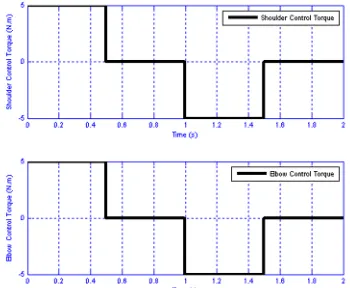
The system has two inputs which are the mechanical shoulder and elbow torques τ t and τ t , and three accessible noisy outputs θ t , θ t , and q t .

The EKF and UKF numerical algorithms were implemented in Matlab environment, while the model simplifying and the jacobians derivation was carried out using the Mathematica packages. The nonlinearities of the process model requires a relatively small time steps for numerical integration. It’s been set to 0.001 s, and the measurement update frequency of the filters coincides with the system discretization sampling frequency.

Table 1: Numerical Parameters of the System

Rigid link

Mass m 1 m·

Length 0.5 9

Inertia 7 0.0834 m·. 9²

Flexible link

Length 0.5 9

Mass density per unit length

;< 0.15 m·. 9›

Flexural

rigidity E7 1 ¤. 9

Quadratic

moment 7 1.45 10›¸ 9¹ First

mode damping coefficient

~ 0.01 9

First mode damping coefficient

ω 36.3131 º&/

Elbow hub Radius 0.04 9

Mass 9₈ 0.5 m·. 9²

Shoulder servomotor

and hub

Inertia 7₈ 0.002 m·. 9²

Elbow servomotor

Viscous friction coefficient

|}

0.95 ¤9. &› _. ›

Table 1 shows the links, hubs and servomotors parameters needed for the numerical simulation, and Figure 2 to Figure 4 show respectively the control torques used for the simulation and the noisy measurement used for the state estimate update for the small noise case and for the large noise case.

ISSN: 1992-8645 www.jatit.org E-ISSN: 1817-3195

717

Figure 3: Nominal and Noisy measurements for the Small Noise Case

Figure 4: Nominal and Noisy measurements for the Large Noise Case

For the two cases, the simulations have been conducted given the following assumptions:

•Both the process noise and the measurement noise are Gaussian, zero-mean, white and with known covariance matrices.

•The EKF and the UKF models used for estimation are always the same, and they are perfectly equal

to the truth model.

•The initial state and process/measurement noise covariances are the same for both the EKF and UKF.

•The truth model initial state is chosen as :

? p ? ? e? % ? % ? e% ?qr

p0q»Ž

While both filters algorithms suppose the following initial state:

•? ‘ ¼? ¼? e• ? ¼%? ¼%? e•%?’

r

p4 4 0.1 2 2 0.2qr

•For the UKF algorithm, the weight coefficients are:

½_!!? 0

¦ _{2# " 1 ⋯ 2#}1

The parameterκ was set to zero.

•The initial error covariance is assumed to be: D 0 •?•?r for the EKF.

D 0 10 7»Ž» for the UKF.

•The process noise and measurement noise covariance matrices are respectiveley given by:

“ 0.1 7»Ž»for the samll noise case.

“ 7»Ž» for the large nois case.

” 0.5 ¾"º·¿Ž¿ 1,1, 10›¹ for the samll noise

case.

” ¾"º·¿Ž¿ 1,1, 10›¹ for the large noise case.

•The update period of the simulation is 0.001 , and the simulation time is 2s.

One can notice from the displayed results that both the EKF and the UKF state estimates converge to the true state.

ISSN: 1992-8645 www.jatit.org E-ISSN: 1817-3195

718

Figure 5: Shoulder Angle Estimation for the Small Noise Case Using the EKF

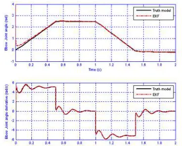
Figure 6: Elbow Angle Estimation for the Small Noise Case Using the EKF

Figure 7: Modal Coordinate Estimation for the Small Noise Case Using the EKF

Figure 8: Shoulder Angle Estimation for the Small Noise Case Using the UKF

Figure 9: Elbow Angle Estimation for the Small Noise Case Using the UKF

ISSN: 1992-8645 www.jatit.org E-ISSN: 1817-3195

719

Figure 11: Shoulder Angle Estimation for the Large Noise Case Using the EKF

Figure 12: Elbow Angle Estimation for the Large Noise Case Using the EKF

Figure 13: Modal Coordinate Estimation for the Large Noise Case Using the EKF

Figure 14: Shoulder Angle Estimation for the Large Noise Case Using the UKF

Figure 15: Elbow Angle Estimation for the Large Noise Case Using the UKF

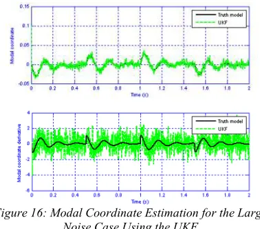
Figure 16: Modal Coordinate Estimation for the Large Noise Case Using the UKF

However, and according to Figures 11 to 16, it’s clear that large noises make the UKF results less accurate, especially when estimating the time derivative state variables.

ISSN: 1992-8645 www.jatit.org E-ISSN: 1817-3195

720

”lÀE ¦ Á 1_¤Â° •¦ ¦

ÃÄ

Ÿ²

39

Where ¤_Â is the number of samples.

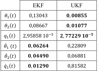
According to the results, displayed by Table 2 and Table 3, a clear performance advantage is demonstrated for the UKF when estimating the shoulder angle, the elbow angle and the modal coordinate, while the EKF is more accurate when estimating their respective time derivatives. This is true either when large or small noises are corrupting the system dynamics or the avilable measurements.

Table 2: Root Mean Square Error for Small Measurements noise

EKF UKF

' 0,02512 Å, ÅÅÆÇÈ

' 0,01877 Å, ÅÅÆÉÊ

e ' 9,08194 10›» _{Ë, ÊÌÆÈÍ ÈÅ}›Ë

% ' 0,01050 Å, ÅÈÅÇÌ

% ' Å, ÅÅÆÊÌ 0,016215

e% ' Å, ÅÅÇÅÉ 0,01344

Table 3: Root Mean Square Error for Large Measurements noise

EKF UKF

' 0,13043 Å, ÅÅÆÌÌ

' 0,08667 Å, ÅÈÅÍÍ

e ' 2,95858 10›Î _{Ç, ÍÍÇÇÊ ÈÅ}›Ì

% ' Å, ÅËÇËÏ 0,22809

% ' Å, ÅÏÏÊÅ 0,06881

e% ' Å, ÅÈÇÊÅ 0,81582

5. CONCLUSION

This paper considers the problem of nonlinear filtering for the 2 Degrees of Freedom (2DOF) Rigid-flexible manipulator state estimation. An exact dynamic model of the manipulator moving in a horizontal plane is derived using the Hamilton’s principle and the assumed modes method considering the first elastic mode.

The paper main contribution is to evaluate the ability of the Extended and Unscented Kalman

filters when used to give a state estimate based on the available noisy measurements. The discussion concerns both the large and small noises assumptions.

According to the simulation results, the required time for the error to converge is lowered with the UKF when the process/measurements noises are assumed to be small. The EKF is better facing large noises.

The RMSE criterion is used to quantify the estimation error. The numerical results demonstrate that the UKF outperforms the EKF when estimating the shoulder angle, the elbow angle and the modal coordinate. The EKF is sensibly more accurate when estimating their respective time derivatives.

REFERENCES

[1] Shitole C. and Sumathi P., “Sliding DFT-based vibration mode estimator for single-link flexible manipulator”, IEEE/ASME Transactions on Mechatronics, Vol. 20, No. 6, 2015, pp. 3249-3256.

[2] Dwivedy S.K. and Eberhard P. “Dynamic analysis of flexible manipulators, a literature review”, Mechanism and Machine, Vol. 41, No. 7, 2006, pp. 749-777.

[3] Mosayebi M., Ghayour M. and Sadigh M.J., “A nonlinear high gain observer based input– output control of flexible link manipulator”,

Mechanics Research Communications, Vol. 45, 2012, pp. 34–41.

[4] Kurode S. and Merchant M., “Observer based control of flexible link manipulator using discrete sliding modes”, Proceedings of IEEE International Conference on Control Application (Hyderabad), August 28-30, 2013, pp. 276–281.

[5] Yang H., Liu J. and Lan X., “Observer design for a flexible-link manipulator with PDE model”, Journal of Sound and Vibration, Vol. 341, No. 14, 2015, pp. 237–245.

[6] Jiang T., Liu J. and He W., “Boundary control for a flexible manipulator based on infinite dimensional disturbance observer”, Journal of Sound and Vibration, Vol. 348, No. 21, 2015, pp. 1-14.

ISSN: 1992-8645 www.jatit.org E-ISSN: 1817-3195

721 [8] Atashzar S.F., Talebi H.A., Towhidkhah F. and

Shahbazi M., “Tracking control of flexible-link manipulators based on environmental force disturbance observer”, Proceedings of the 49th IEEE Conference on Decision and Control, (Atlanta, GA), December 15-17, 2010, pp. 3584–3589.

[9] Simon D., “Optimal State Estimation: Kalman, H Infinity, and Nonlinear Approaches”, John Wiley & Sons, Inc, 2006.

[10] Kushner H.J., “Dynamical equations for optimal nonlinear filtering”, Journal of Differential Equations, Vol. 3, No. 2, 1967, pp. 179–190.

[11] Walpole R.E., Myers R.H., Myers S.L., and Ye K., “Probability & Statistics for Engineers & Scientists”, Prentice Hall, Boston, 2012. [12] Chui C.K. and Chen G., “Kalman filtering

with real-time applications”, Springer, Berlin, 2009.

[13] Julier S.J. and Uhlmann J.K., “Unscented filtering and nonlinear estimation”,

Proceedings of IEEE, Vol. 92, No. 3, 2004, pp. 401-422.

[14] M. BAKHTI & B. B. IDRISSI, “Highly Nonlinear Flexible Manipulator State Estimation Using the Extended and the Unscented Kalman Filters”, International Review of Automatic Control (IREACO), Vol.9, No.03, 2016, pp. 151-160.

[15] M. BAKHTI & B. B. IDRISSI, “Nonlinear One Link Flexible Manipulator State Estimation Using the Extended Kalman Filter”, International Journal of Control and Automation, Vol. 9, No. 11, 2016, pp. 315-326.

[16] M. BAKHTI & B. B. IDRISSI, “Active Vibration Control of a Flexible Manipulator Using Model Predictive Control and Kalman Optimal Filtering“, International Journal of Engineering Science and Technology, Vol. 5, No. 1, 2013, pp. 165-177.

[17] Tokhi M.O. and Azad A.K.M. “Flexible Robot Manipulators Modelling, simulation and control”, The Institution of Engineering and Technology, 2008.

[18] Yigit A.S., Scott R.A., and Ulsoy A.G., “Flexural motion of a radially rotating beam attached to a rigid body”, Journal of Sound and Vibration, Vol. 121, No. 2, 1988, pp. 201-210.

[19] Dym C. L. and Shames I. H., “Solid mechanics, a variational approach”, Springer, New York, 2013.

[20] Hassan M., Dubay R., Li C. and Wang R., “Active vibration control of a flexible one-link manipulator using a multivariable predictive controller”, Mechatronics, Vol. 17, No. 6, 2007, pp. 311–323.

ISSN: 1992-8645 www.jatit.org E-ISSN: 1817-3195

722

APPENDIX

MODEL MATRICES AND VECTORS EXPRESSIONS WITH NUMERICAL VALUES

The elements of the symmetric mass matrix:

l e ‘9¦Ð’_¿Ž¿

9 78 : ;<=> &

? ;<

2 /1_{2 ;<} ;< 0

7 98

2 "# F: ;<f=> &

? H e

9 0.2370  0.0218 cos 0.08e sin

9 78 : ;<=> &

?

/1_{2 ;<} ;< 0

"# F: ;<f=> &

? H e

9 0.0099  0.0109 cos 0.04e sin

9 ¿ : ;< f &

=>

?

F: ;<f=> &

? H

9 ¿ 0.0323 0.04 cos

9 78 : ;<=> &

?

9 0.0099

9 ¿ : ;< f &

=>

?

9 ¿ 0.0323

9¿¿ : ;<+f=> , & ?

9¿¿ 0.1392

The elements of the diagonal stiffness matrix:

m e ‘³¦Ð’_¿Ž¿

³ ³ 0

³¿¿ : E7 F=> G †_{G H &} ?

³¿¿ 183.52

The elements of vector:

i e, e% pi¦q¿Ž

i

Ò/1_{2 ;<} ;< 0 sin

F: ;<f=> &

? H e Ó %

F2 /1_{2 ;<} ;< 0 "#

2 F: ;<f=> &

? H e H % %

2 "# ÒF: ;<f=> &

? H e% Ó + % % ,

i % 0.04e cos 0.0109 sin

% % e cos 0.0218 sin

0.08+ % % ,sin

i

Ò/1_{2 ;<} ;< 0 sin

F: ;<f=> &

? H e Ó %

i % 0.04 e 0.0109 "#

i¿

F: F;<=> f` f ?

1

2 ;< 2 2 f`` f H & 78

: ;<=> &

? ;<

2 /1_{2 ;<} ;< 0 7 98

2 "# F: ;<f=> &

? H e H e + % % ,

F: ;<f=> &

? H e sin θ θ

i¿ 0.0444 e % % 0.04 % sin

The elements of the diagonal damping matrix:

z{ e ‘i&¦Ð’_¿Ž¿

i& i& 0.95