BIROn - Birkbeck Institutional Research Online
Psaradakis,
Zacharias
(2017)
Markov-Switching
Models
with
state-dependent time-varying transition probabilities. Working Paper. Birkbeck
College, University of London, London, UK.
Downloaded from:
Usage Guidelines:
Please refer to usage guidelines at or alternatively
ISSN 1745-8587
Department of Economics, Mathematics and Statistics
BWPEF 1702
Markov-Switching Models with
State-Dependent Time-Varying
Transition Probabilities
Zacharias Psaradakis
Birkbeck, University of London
Martin Sola
Universidad Torcuato di Tella, Argentina
March 2017
Birkb
eck Worki
ng
Papers i
n
Economi
cs
&
Fina
Markov-Switching Models with State-Dependent
Time-Varying Transition Probabilities
∗
Zacharias Psaradakis
Department of Economics, Mathematics and Statistics,
Birkbeck, University of London, U.K.
Martin Sola
Department of Economics, Universidad Torcuato di Tella, Argentina
March 2017
Abstract
This paper proposes a model which allows for discrete stochastic breaks in the
time-varying transition probabilities of Markov-switching models with autoregressive
dy-namics. An extensive simulation study is undertaken to examine the properties of the
maximum-likelihood estimator and related statistics, and to investigate the
implica-tions of misspecification due to unaccounted changes in the parameters of the Markov
transition mechanism. An empirical application that examines the relationship
be-tween Argentinian sovereign bond spreads and output growth is also discussed.
Keywords: Markov-switching models; Maximum likelihood; Monte Carlo experiments;
Time-varying transition probabilities.
JEL Classification: C32.
∗The authors wish to thank Demian Pouzo for helpful discussions and suggestions. Address
1
Introduction
Since the publication of Diebold, Lee, and Weinbach (1994) and Filardo (1994), time-series
models with parameters which are subject to changes governed by a finite-state Markov
chain with time-varying transition probabilities have attracted considerable attention in
the literature. Applications involving such models can be found in many areas of economics
and finance. Examples include, among many others, the study of business-cycle fl
uctua-tions (Filardo (1994); Filardo and Gordon (1998); Ravn and Sola (1999)), exchange rates
(Diebold, Lee, and Weinbach (1994); Engel and Hakkio (1996)), interest-rate dynamics
(Bekaert and Harvey (1995); Gray (1996)), asset allocation (Bekaert and Harvey (1995);
Ang and Bekaert (2002); Guidolin and Timmermann (2006); Guidolin and Timmermann
(2008)), asset returns (Hall, Psaradakis, and Sola (1997); Schaller and van Norden (1997)),
andfinancial/exchange-rate crises (Jeanne and Masson (2000); Peria (2002); Alvarez-Plata
and Schrooten (2006); Brunetti, Scotti, Mariano, and Tan (2008)).
A question which is often addressed in empirical studies using regime-switching models
with time-inhomogeneous Markov transitions is which variables help to predict the
tran-sitions between different regimes (a period of relative calm and a financial crisis, say). In
such applications the sample typically includes data from all regimes and one of the objects
of the exercise is to separate the regimes on the basis of sample information. An implicit
assumption usually made is that the association between the information variables that
enter in the transition probabilities and the dependent variable of the model is not altered
by the regime changes, so that the parameters associated with the transition probabilities
are time invariant.
However, this may not necessarily be a plausible assumption in some empirical
appli-cations. Ravn and Sola (1999), for instance, observed that a change in the definition of M2
money stock in the U.S., and therefore in the correlation between M2 and output growth,
had a dramatic impact on regime separation. When they considered a short sample which
ended before the change in the definition of M2, they found the separation of regimes into
booms and recessions to be consistent with the National Bureau of Economic Research
significant effect on the transition probabilities. When the sample was extended, M2 no
longer had a significant effect on the transition probabilities and the separation of regimes
was unrelated to the NBER dating. In view of the fact that in many applications the
reason for including exogenous variables in the transition mechanism is to use them as
leading indicators of a given event (e.g., a financial crisis), the problem just described
is likely to be the rule rather than the exception. As a result, it is likely that
poten-tial leading indicators may be found in applications to have no significant effect on the
transition probabilities, or may be found to be significant because of the strength of their
covariation with the dependent variable after the event (which could not justify their use
as leading indicators of the event). In addition, it is likely that the in-sample separation
of the regimes will be adversely affected and lead to misleading conclusions.
The contribution of this paper is to propose a regime-switching model which explicitly
allows for random breaks in the time-inhomogeneous transition probability matrices of the
hidden Markov regime sequence. We conjecture that a change in the (nonlinear)
relation-ship between the variable being modelled and the information variables that determine
the evolution of the transition matrices, is likely to result in changes in the covariance
between these variables as well as in the relationship between the information variables
and the transition probability matrices. Therefore, we propose to consider a
multivari-ate model (e.g., a vector autoregression with Markov regimes) in which both the noise
covariance matrix and the transition functions are subject to random breaks driven by
an exogeneous finite-state Markov process. In many applications in which an
informa-tion variable (e.g., money supply) is used as a leading indicator (e.g., of an exchange-rate
crisis), although the covariation between the information variable and the main variable
of interest (e.g., exchange rate) is likely to have changed over the sample period, the
po-tential resulting changes in the parameters associated with the transition mechanism and
the noise covariance matrix are rarely taken into account. The principal idea behind our
modelling strategy is to use such breaks to identify changes in the (indirect) relationship
between the time series of interest and the transition information variable(s). Our
on likelihood-based statistical inference.
The remainder of the paper is organized as follows. Section 1 recalls the structure of
a typical Markov-switching autoregressive model and motivates our modelling approach.
Section 2 introduces and discusses the proposed multivariate model. Section 3 contains
a simulation study that assesses the properties of estimators and test statistics in the
presence of parameter changes in the Markov transition functions. Section 4 presents
an illustrative empirical application that analyzes the relationship between Argentinian
sovereign bond spreads and output growth. Section 5 summarizes and concludes.
2
Markov-Switching Models and Motivation
A prototypical Markov-switching autoregressive model for a univariate time series{Yt} is
given by
Yt=μ(St) +φ0yt−1+σ(St)εt, t= 1,2, . . . , (1)
where yt−1 := (Yt−1, . . . , Yt−k)0 for some positive integer k, φ := (φ1, . . . , φk)0 is an
un-known parameter, {εt} are independent, identically distributed (i.i.d.) standard normal
random variables, and {St} are random variables which take values in the setS:={0,1}
and indicate the unobservable state, or regime, prevailing at each pointt. Here and in the
sequel, we write
b(V) :=b0+ (b1−b0)I{V=1},
for any real-valued quantityb(V) whose values depends on the realization of anS-valued
random variableV,I{·}being an indicator variable (withI{A} = 1if conditionAis satisfied
and I{A} = 0 otherwise). The regime-determining variables {St} in (1) are assumed to
be independent of {εt} and to form a time-inhomogeneous Markov chain with transition
probabilities
P(St= 0|St−1 = 0, Zt−1) =:qt=Λ
¡
αq+βqZt−1
¢
, (2)
P(St= 1|St−1= 1, Zt−1) =:pt=Λ(αp+βpZt−1). (3)
where Λ(u) := 1/(1 +e−u) is the standard logistic function and Zt−1 is an exogenous
(1994)). Needless to say, such a model may be straightforwardly generalized to allow
for state-dependent autoregressive coefficientsφ, more than two regimes, and more than
one information variable in (2)—(3); furthermore, Λ(·) may be replaced by some other
continuous, monotonic function whose range lies in the interval[0,1].
Under the formulation in (1)—(3), the observable variable Zt−1 influences the
prob-ability with which {Yt} switches between the two states. This allows for a nonlinear
relationship between Yt and Zt, since Zt−1 affects Yt indirectly through the transition
probabilities pt and qt. Furthermore, the effect of Zt−1 on the transition probabilities
need not be symmetric, in the sense thatβq and βp are not required to be equal or have
the same sign. A Markov-switching autoregressive model with a time-invariant transition
mechanism is, of course, a special case of (1)—(3) withβq =βp = 0.
An important issue which has not received much attention in the literature concerns the
effects on inference of potential changes in the parameters associated with the time-varying
transition probabilities. For example, a number of empirical studies have documented that
several monetary relationships display instability because of changes in monetary policy
and in innovations in the financial sector (see, e.g., Ravn and Sola (1999)). Such changes
may lead to instability in the parameters associated with the transition probabilities and
may have deleterious effects on inference if they are not accounted for.
A simple set-up, investigated in Psaradakis, Sola, Spagnolo, and Spagnolo (2013),
allows the Markov chain {St} in (1) to be governed by the transition probabilities
qt=Λ
¡
αq+βq,tZt−1
¢
, pt=Λ
¡
αp+βp,tZt−1
¢
, (4)
where, for some fixed integer t∗ >1,
βi,t =βi+ (β∗i −βi)I{t−t∗>0}, i=p, q, t>1. (5)
Under the formulation (4)—(5), the relationship between the transition probabilities and
the variable Zt−1 undergoes an one-off change at t = t∗. In such a case, the transition
mechanism (2)—(3) is misspecified when β∗q−βq 6= 0 and/or β∗p−βp 6= 0, and inference
A more general formulation, which can accommodate stochastic changes in the
tran-sition probabilities at unspecified dates, may be obtained by allowing the parameters
(αq, αp, βq, βp) in (2)—(3) to vary as a time-homogeneous,finite-state Markov chain.
Un-der such a formulation, the relationship between the transition probabilities of {St} and
the variableZt−1 undergoes discrete random changes. A multivariate model which allows
for such behavior is discussed next.
3
Modelling Breaks in the Markov Transition Mechanism
For simplicity and clarity of exposition, we will present and discuss in the sequel a bivariate
model. The model aims to capture changes in the relationship between Yt and Zt by
conjecturing that such changes would manifest as changes in the covariance structure
between Yt and Zt and in the transition mechanism of {St}. This covariance structure,
as well as the time-varying transition probabilities of {St}, are then modelled as being
subject to random breaks governed by an exogenousfinite-state Markov process.
3.1
Model
Let{vt}be an unobservable sequence of i.i.d. random vectors having a bivariate standard
normal distribution and {ξt:= (St, Xt)0} be an unobservable sequence of random vectors
taking values inS×S. We consider the following model for the observable bivariate time
series {wt:= (Yt, Zt)0}:
Yt=μ(St) +φ0yt−1+σ(St)εyt, t= 1,2, . . . , (6)
Zt=μz+ψ0zt−1+σzεzt, t= 1,2, . . . , (7)
whereyt−1 := (Yt−1, . . . , Yt−k)0 and zt−1 := (Zt−1, . . . , Zt−m)0 for some positive integersk
and m,φ:= (φ1, . . . , φk)0 and ψ:= (ψ1, . . . , ψk)0 are unknown parameters, and the noise
εt:= (εyt, εzt)0 satisfies
εt=R1t/2vt, (8)
Rt=
⎡
⎣ 1 ρ(Xt)
ρ(Xt) 1 ⎤
⎦, (9)
and |ρi|< 1,i∈ S. The model is completed by postulating that, conditionally on {Xt},
{St} is a time-inhomogeneous Markov chain whose transition probabilities depend on
(Zt−1, Xt) and have the following functional form:
P(St= 0|St−1 = 0, Zt−1, Xt) =:qt(Xt) =Λ
¡
αq(Xt) +βq(Xt)Zt−1
¢
, (10)
P(St= 1|St−1= 1, Zt−1, Xt) =:pt(Xt) =Λ
¡
αp(Xt) +βp(Xt)Zt−1
¢
. (11)
In addition, {Xt}is a time-homogeneous Markov chain with transition probabilities
P(Xt= 0|Xt−1= 0) =qx, P(Xt= 1|Xt−1 = 1) =px. (12)
Finally,{ξt},{vt}andw0:= (y00,z00)0are independent of each other, andXtis independent
of {Sr:r < t}for all t.
Under the formulation (6)—(12), the covariance structure of wt, as captured by the
covariance matrixRt, is subject to Markov changes governed by{Xt}. At the same time,
the transition mechanism that governs the Markov process{St}driving the changes in the
conditional mean and variance of{Yt}is also dependent upon the state of nature implied
by {Xt}. The model may, of course, be generalized to allow for more than two states
and/or variables, as well as state-dependent parameters(φ,ψ, μz, σz).
3.2
Estimation and Inference
Given data w0,w1, . . . ,wT, statistical inference in the model defined by (6)—(12) can be
carried out by using a recursive algorithm analogous to that discussed in Hamilton (1994,
pp. 692—694). This entails iterating on the equations
δt|t= [10(δt|t−1¯ηt)]−1(δt|t−1¯ηt), t= 1,2, . . . , T, (13)
and
where
δt|τ :=
⎡ ⎢ ⎢ ⎢ ⎢ ⎢ ⎣
P[ξ0t= (0,0)|Fτ;θ] P[ξ0t= (0,1)|Fτ;θ] P[ξ0t= (1,0)|Fτ;θ] P[ξ0t= (1,1)|Fτ;θ]
⎤ ⎥ ⎥ ⎥ ⎥ ⎥ ⎦
, ηt:=
⎡ ⎢ ⎢ ⎢ ⎢ ⎢ ⎣
f00(wt|ξ0t= (0,0),Ft−1;θ)
f01(wt|ξ0t= (0,1),Ft−1;θ) f10(wt|ξ0t= (1,0),Ft−1;θ)
f11(wt|ξ0t= (1,1),Ft−1;θ)
⎤ ⎥ ⎥ ⎥ ⎥ ⎥ ⎦ , and Pt:= ⎡ ⎢ ⎢ ⎢ ⎢ ⎢ ⎣
qt0qx qt0(1−px) (1−pt0)qx (1−pt0)(1−px)
qt1(1−qx) qt1px (1−pt1)(1−qx) (1−pt1)px
(1−qt0)qx (1−qt0)(1−px) pt0qx pt0(1−px) (1−qt1)(1−qx) (1−qt1)px pt1(1−qx) pt1px
⎤ ⎥ ⎥ ⎥ ⎥ ⎥ ⎦ .
Here,θ denotes the (column) vector of all parameters of the model,Ft:={wr:r 6t} is
the information set available at timet,fij(wt|ξ0t= (i, j),Ft−1;θ)is the conditional density
of wt given ξ0t= (i, j), i, j∈S, andFt−1,1 is a four-dimensional all-ones column vector,
and ¯denotes element-wise multiplication.
Note that, under the Gaussianity assumption forvt,fij(wt|ξ0t= (i, j),Ft−1;θ),i, j∈S,
is the bivariate normal density with mean vector
¡
μ0+ (μ1−μ0)i+φ0yt−1, μz+ψ0zt−1
¢0
and covariance matrix ⎡
⎣ σ20+ (σ21−σ20)i σz{σ0+ (σ1−σ0)i}{ρ0+ (ρ1−ρ0)j}
σz{σ0+ (σ1−σ0)i}{ρ0+ (ρ1−ρ0)j} σ2z
⎤ ⎦.
Also note that one may think of the model (6)—(12) as allowing for four Markov states,
which may be indexed by the state-indicator variable
ζt:=
⎧ ⎪ ⎪ ⎪ ⎪ ⎪ ⎨ ⎪ ⎪ ⎪ ⎪ ⎪ ⎩
1, if ξ0t= (0,0),
2, if ξ0t= (0,1),
3, if ξ0t= (1,0),
4, if ξ0t= (1,1).
Then, {Pt} may be regarded as the time-inhomogeneous transition probability matrices
of the Markov chain {ζt}, the (i, j)-th element of Pt being the transition probability
The algorithm based on the iteration of (13)—(14) yields as a by-product the conditional
log-likelihood of (w1, . . . ,wT), given (w0,ξ0):
(θ) := T
X
t=1
ln[10(δt|t−1¯ηt)]. (15)
The maximum-likelihood (ML) estimator bθ of the parameter θ can then be obtained as
the maximizer of (15) with respect toθ. Furthermore, inference about the hidden regimes
{ξt}may be made on the basis of the smoothed state probabilitiesδt|T or thefiltered state
probabilities δt|t (evaluated atθ =bθ).
Asymptotic results relating to consistency and local asymptotic normality of the ML
estimator of the parameters of Markov-switching autoregressive models with time-varying
transition probabilities were recently established in Pouzo, Psaradakis, and Sola (2016).
Under the assumption of correct model specification and suitable stationarity, ergodicity,
identification and moment conditions, the usual asymptotic theory for the ML estimator
holds in a model like (6)—(12). In particular,bθis consistent and asymptotically efficient for
the true parameter θ0 (say), and [−¨(bθ)]1/2(bθ−θ0) has a Gaussian limiting distribution
with zero mean vector and identity covariance matrix, as T tends to infinity, where ¨(bθ)
is the Hessian matrix of (θ) evaluated at θ =bθ. In the presence of specification errors,
and under certain regularity conditions, bθ is consistent for the parameter that provides
the best approximating model, in the sense of minimizing the Kullback—Leibler divergence
from the true data-generating process (DGP).
4
Monte Carlo Simulations
Simulation experiments are carried out to assess the properties of the ML estimator and of
related test statistics both in correctly specified models and in misspecified models which
ignore changes in the parameters associated with the Markov transition functions. We
begin by describing the experimental design and simulations, and proceed to report and
4.1
Experimental Design and Simulation
The DGP used in the experiments is the bivariate model defined by (6)—(12), with fi
rst-order dynamics(k=m= 1) and the following parameter values:
μ0= 3, μ1= 0.5, φ= 0.9, σ0= 0.5, σ1= 1,
μz = 0.1, ψ= 0.8, σz = 1, ρ0 = 0.8, ρ1 =−0.8,
px =qx = 0.95, αp0 =αp1 = 1, αq0=αq1 = 2,
[image:12.595.96.524.325.480.2]βq0 =−1.5, βq1 = 3, βp0= 2.5, βp1 =−5.
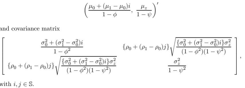
Figure 1 shows the regime-specific marginal densities of wt, that is, bivariate normal
densities having mean vector µ
μ0+ (μ1−μ0)i
1−φ , μz
1−ψ
¶0
and covariance matrix ⎡ ⎢ ⎢ ⎢ ⎢ ⎣
σ20+ (σ21−σ20)i
1−φ2 {ρ0+ (ρ1−ρ0)j}
s
{σ20+ (σ21−σ20)i}σ2z
(1−φ2)(1−ψ2)
{ρ0+ (ρ1−ρ0)j}
s
{σ20+ (σ21−σ20)i}σ2z
(1−φ2)(1−ψ2)
σ2z
1−ψ2
⎤ ⎥ ⎥ ⎥ ⎥ ⎦,
withi, j∈S.
In each of 1000 Monte Carlo replications, we generate 100 +T data points for wt,
with T ∈ {100,200,400,800,1600,3200,6400} and w00 = (0.5,0.40118), but only the last
T data points of each realization are used in order to attenuate start-up effects. For each
realization, we compute ML estimates of the parameters of three bivariate models for
(Yt, Zt): (i) a model defined by (6)—(9), withρ(Xt) = ρfor all t, coupled with the
state-independent Markov-switching mechanism associated with (2)—(3) (model M-1); (ii) the
model defined by (6)—(12) with both{St}and{Xt}treated as unobservable (model M-2);
(iii) a model defined by (6)—(12), but with the additional assumption that the realization
of the Markov process {Xt}driving the changes in the transition probabilitiesqt(Xt)and
pt(Xt)of{St}and the covariance matrixRtis observable (model M-3). We setk=m= 1
Model M-1 is evidently misspecified since it ignores the breaks in the covariance matrix
of εt and in the transition probabilities of {St}. Model M-3 accounts for the Markov
breaks in qt(Xt), pt(Xt) and ρ(Xt) correctly, but an observable regime sequence {Xt} is
not typically available in situations involving real-world data. However, a comparison of
parameter estimates obtained from model M-3 and the empirically relevant model M-2
will reveal whether the ML estimator suffers as a result of the additional randomness
introduced by the Markov process{Xt}.
For all three models, the maximizer of the relevant ML objective function is found
by means of a quasi-Newton algorithm that approximates the Hessian according to the
Broyden—Fletcher—Goldfarb—Shanno (BFGS) update with numerically computed
deriva-tives. A grid of seven initial values for each parameter is used to initialize the BFGS
iterations; those initial values which result in the highest value of the objective function
are then selected.1
Figure 2 shows plots of: a typical realization of{Yt}and{Zt}; the time-varying
transi-tion probabilitiespt(Xt)andqt(Xt)and their estimated values (the latter are computed as
¯
pt=P(Xt= 0|Ft)p0t+P(Xt= 1|Ft)p1t andq¯t=P(Xt= 0|Ft)q0t+P(Xt= 1|Ft)q1t); the
associated realizations of the Markov chains{St}and{Xt}; thefiltered state probabilities
P(St = 1|Ft;θb) and P(Xt= 1|Ft;bθ); all quantities depending on the unknown parameter
θ are computed using the ML estimatorbθ from model M-2. For this typical realization,
model M-2 is remarkably successful at capturing the changes in regime and the movements
in the transition probabilities of {St}. It is interesting to compare results for the same
realization of{Yt}and{Zt}when model M-1 is used instead. The relevant plots, shown in
Figure 3, reveal that, although model M-1 is equally successful in identifying the changes
in regime associated with {St}, it fails dramatically in describing the dynamics ofpt(Xt)
and qt(Xt). This suggests that it is unlikely that Zt−1 would be found to be useful in
predicting the shifts implied by the regime sequence {St}. As we shall see below, this is
not a peculiar feature of the particular realization used in Figure 3 but is true in general.
1
4.2
Simulation Results
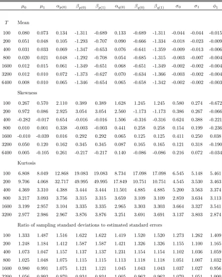
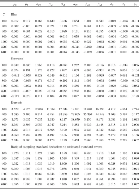
Table 1a records some of the characteristics of the finite-sample distribution of the ML
estimator of the parameters of the equation for Yt in model M-1. Specifically, we
re-port the estimated bias and conventional measures of skewness and kurtosis based on the
standardized third and fourth empirical central moments. We also report the ratio of
the sampling standard deviation of the ML estimators to the estimated standard errors
(computed from the empirical Hessian) averaged across Monte Carlo replications for each
design point. Note that in Table 1a (as well as in Tables 1b and 1c) the figures reported
underαp(i),βp(i),αq(i)andβq(i),i∈S, refer to deviations of the ML estimates of the
para-meters(αp, βp, αq, βq)in (2)—(3) from the true regime-specific values of the corresponding
parameters. The most noteworthyfinding is the significant bias in the estimation of
para-meters associated with the transition probabilities, especiallyβq and βp. Such biases are
clearly not a small-sample issue and are present even in the largest of the samples under
consideration (T = 6400). For small sample sizes (T 6 200), the distributions of the
estimators of many parameters tend to be asymmetric and leptokurtic, but the situation
improves with increasing sample sizes. Finally, the estimated standard errors are
down-wards biased in most cases; however, the bias is not generally substantial and decreases
as the sample size increases.
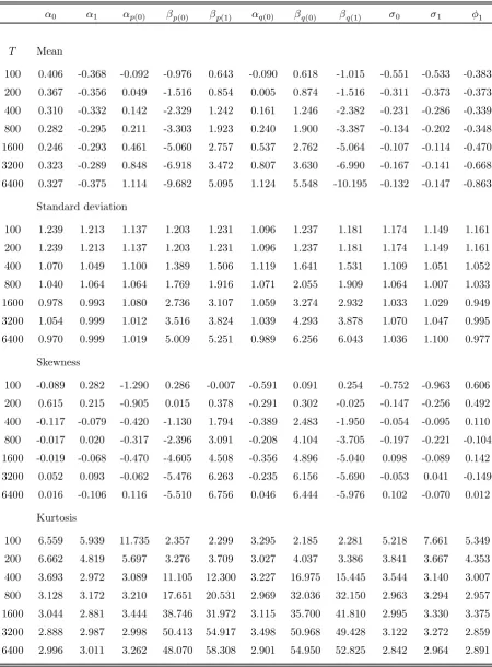
Table 1b contains information on the sampling distributions of conventional t-type
statistics, computed as the ratio of the estimation error to the corresponding asymptotic
standard error, and are typically treated as having an approximate standard normal
dis-tribution (which is true under the assumption of a correctly specified likelihood function).
It is immediately obvious that the mean of these distributions can differ substantially from
zero, something which is especially true for t-statistics associated with the parameters of
the transition functions. The studentized statistics generally tend to have skewed
distrib-utions and, in the case of βq and βp, highly leptokurtic (especially for the larger sample
sizes).
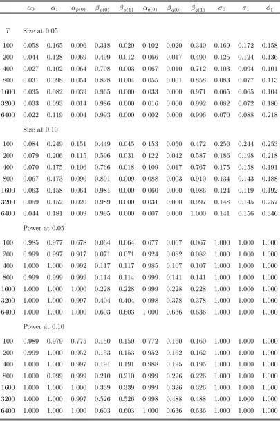
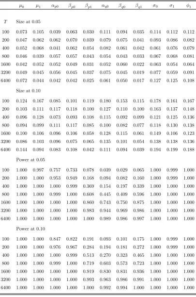
To examine the implications of these results for hypothesis testing, we report in
nominal size 0.05 and 0.10) of: (i) at-type test ofH0 :ϑj =ϑ∗j versusH1 :ϑj 6=ϑ∗j, where
ϑj is the j-th element of the parameter vector ϑ of the model under consideration and
ϑ∗j is its true value; (ii) a t-type test of H0 :ϑj = 0 versus H1 : ϑj 6= 0; we refer to the
estimated rejection frequencies as ‘size’ and ‘power’, respectively.2 It can be seen that the
hypothesis thatβqorβpis equal to either of the two regime-specific true values is rejected
either very rarely or very frequently. Furthermore, tests for the statistical significance of
these parameters have very low power. As a result, one may be wrongly led to conclude
that a significant leading indicator has no effect on the Markov transition probabilities.
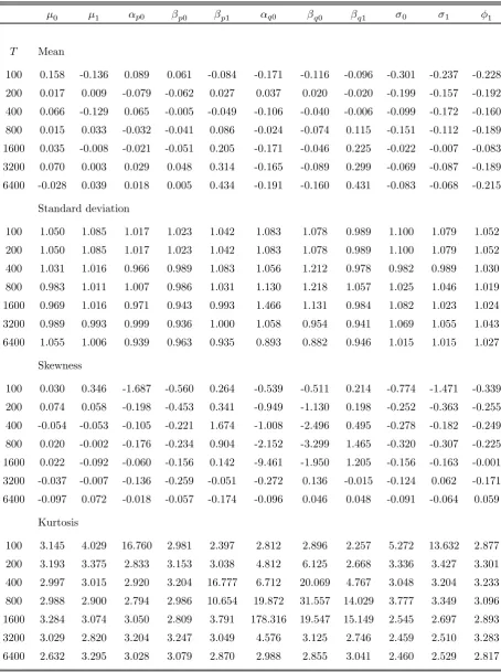
Table 2a records some of the characteristics of thefinite-sample distribution of the ML
estimator of the parameters of the equation for Yt in the well-specified model M-2. In
sharp contrast to the results obtained under model M-1, the ML estimator exhibits some
bias only in small samples and, even for the parameters associated with the transition
probabilities, bias is insignificant for T > 400. The distributions of the estimators of
some parameters tend to be asymmetric and leptokurtic, but the situation improves with
increasing sample sizes. Finally, the bias in the estimated standard errors is not generally
substantial and decreases as the sample size increases.
Encouraging results are also contained in Table 2b, in which information on the
empir-ical distributions of conventional t-type statistics is recorded. The studentized statistics
tend to have distributions with mean and variance that do not differ substantially from
their expected values in most cases. Rather surprisingly, the mean of the studentized
statistics associated with βq1 and βp1 is significantly different from zero when T >1600.
This, however, does not appear to have an adverse effect on the size and power
proper-ties of t-type tests, the empirical rejection frequencies of which are reported in Table 2c.
Unlike the case of model M-1, tests in model M-2 tend to have an empirical Type I error
probability which is generally close to the nominal level of the test, especially forT >200.
In terms of power, tests involving the parameters associated with the time-varying
transi-tion probabilities tend to fare somewhat worse than tests involving other parameters, but
rejection frequencies improve with an increasing sample size.
2We note that results should be interpreted with caution in the case of
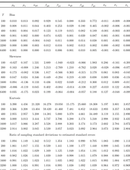
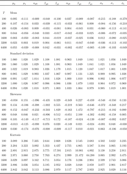
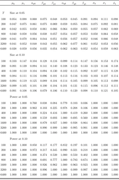
The simulation results reported in Tables 3a—3c for model M-3 are generally quite
sim-ilar to those obtained under model M-2. Perhaps the only noteworthy difference concerns
the mean of the studentized statistics associated withβq1 andβp1, which is closer to zero
under model M-3. It is worth emphasizing that model M-3 is not empirically relevant
since it assumes that the changes in the Markov transition probabilities and the noise
covariance matrix are observable. The simulation results, however, do suggest that not
much is lost by treating the aforementioned breaks as unobservable random events driven
by an exogeneous Markov process.
To sum up, the results from the Monte Carlo experiments suggest that, in the
pres-ence of unaccounted changes in the parameters of the transition functions and the noise
covariance matrix, ML produces severely biased estimates, especially for the parameters
that appear in the transition probabilities. Such biases are present even for what are very
large sample sizes by the standards of empirical applications. Hypothesis tests based on
such ML estimates also have unsatisfactory properties. By contrast, the ML estimator in
a correctly specified model that allows for hidden breaks in the transition functions and
the noise covariance matrix has very good finite-sample properties and performs almost
as well as a ML estimator which has full knowledge of the number and location of such
breaks.
5
Empirical Application
To illustrate the practical use of the proposed model, we analyze the relationship between
Argentinian sovereign bond spreads over U.S. Treasury rates and output growth. These
variables are generally expected to be negatively correlated since the higher output growth
is, the higher is the capacity of a country to repay debt, leading to lower bond spreads.
However, if a structural break occurs as a result of a default on sovereign debt, then
correlation will typically change because the economy may start to grow after the default,
as resources are no longer used to service the debt, while the country’s risk continues to
increase, resulting in higher bond spreads. It is likely that such a change in correlation
The data set consists of quarterly observations, from 1995:1 to 2010:1, on the J. P.
Morgan Emerging Markets Bond Index (EMBI) of dollar-denominated sovereign bonds
issued by Argentina (denoted byYt) and the real GDP growth rate (denoted byZt). The
focus of the analysis is on whether output growth has predictive content for regime changes
associated with the bond spread in the presence of a potential break in the relationship
between the two variables associated with the sovereign default.
We consider two models. Model 1 is the standard model, à la Diebold, Lee, and
Weinbach (1994), given by (1)—(3). Model 2 is given by (6)—(12), and allows for stochastic
discrete breaks in the noise covariance matrix and in the transition functions. In both
cases, we setk=m= 4.
Model 1 is used because of its popularity in applied work. It should be borne in
mind, however, that, even in the absence of breaks in the transition mechanism and
the noise covariance matrix, the use of such a specification is problematic if Yt and Zt
are contemporaneously correlated, as the analysis in Pouzo, Psaradakis, and Sola (2016)
demonstrates.
ML estimates of the parameters of the two models are reported in Table 4. The
esti-mated coefficients for the Markov transition functions for Model 1, show that an increase
(decrease) in output growth increases (decreases) the probability of remaining in a
high-volatility regime (high output growth and high spread high-volatility) since both βq and βp
are positive and would appear to be statistically significant at the 10% level. We note,
however, that inference based on these ML estimates is potentially misleading because of
the likely bias of the parameter estimator and the inconsistency of the empirical Hessian
covariance estimator in the presence of changes in the parameters of the Markov transition
functions and/or endogeneity of the transition information variable.
The results for Model 2 show that the estimated values of βq0 and βq1 have different
signs, so one would expect the evolution ofqtimplied by Model 1 and Model 2 to be quite
different. A similar result is obtained for βp0 and βp1, the main difference being that in
this case the estimates are both positive and thus one would not expect the evolution of
estimated ρ0 and ρ1 have opposite signs, which suggests that the model is capable of
identifying the expected characteristic of pre-default and post-default periods mentioned
earlier.
Figure 4 shows plots of the estimated time-varying transition probabilities qt and pt
associated with the regimes{St}, as well as thefiltered state probabilitiesP(St= 1|Ft;θb),
for Model 1. We also compute the estimate of the quantity κt := (1−qt)/(2−qt−pt),
which may be thought of as a proxy for the probability thatSt= 1, given currently
avail-able information onZt−1, and gives an indication of the contribution ofZt−1 in predicting
regime changes. It is immediately obvious that the evolution of qt and pt mimics the
movements in the output growth rate and does not seem to be particularly informative
regarding shifts to the regime that is associated with high EMBI. Furthermore, the
move-ments inκt appear to be unrelated to the movements in P(St= 1|Ft;bθ), suggesting that
output growth does not have much predictive ability for regime changes.
For Model 2, Figure 5 shows plots of the estimated time-varying transition probabilities
¯
pt = P(Xt = 0|Ft)p0t+P(Xt = 1|Ft)p1t and q¯t = P(Xt = 0|Ft)q0t+P(Xt = 1|Ft)q1t
(evaluated at θ =bθ) associated with the regime sequence {St}, the quantity ¯κt := (1−
¯
qt)/(2−q¯t−p¯t), and thefiltered probabilities P(St = 1|Ft;bθ) and P(Xt = 1|Ft;θb). The
main difference with Model 1 is that both q¯tandκ¯tnow seem to be informative about the
regime changes associated with EMBI, tracking the movements of P(St = 1|Ft;bθ) more
closely and preceding its changes on several occasions.
The filtered probabilities P(St = 1|Ft;bθ) associated with high EMBI values are very
similar for both models. For Model 1 (Model 2), the (implied) variance of EMBI in the
regime associated withSt = 1 (which includes the default on sovereign debt) is
approxi-mately 12 times (11 times) larger than it is in the regime associated withSt= 0. For Model
1, the (implied) long-run mean of EMBI is 0.7618 (761.8 points since the series was divided
by 1000 prior to estimation) in the regime associated with St = 0 and 3.69997 (3699.9
points) in the regime associated with St = 1; the corresponding figures for Model 2 are
0.3795 (379.5 points) and 1.9083 (1908.3 points), respectively. Finally, the filtered
associated with positive correlation between output growth and EMBI (Xt = 1) and a
regime that is characterized by negative correlation (Xt= 0).
6
Summary
We have considered a class of Markov-switching models with time-varying transition
prob-ability matrices in which the parameters associated with the latter are subject to random
changes driven by an exogenous Markov process. Such changes will typically be related to
changes in the covariance structure between the time series of interest and the information
variables which drive the evolution of the Markov transition probabilities. A simulation
study has demonstrated the pitfalls of ignoring such changes, pitfalls which include biased
parameter estimates and hypotheses tests which exhibit level distortions and low power.
The simulations have also shown that the proposed model and related parameter estimator
share the same desirable characteristics with a model which incorporates perfect
informa-tion about the number and locainforma-tion of the breaks associated with the Markov transiinforma-tion
functions. As an illustration of the practical use of the proposed class of models, we have
analyzed the relationship between sovereign bond spreads and output growth in Argentina.
The correlation structure between these two variables, and hence the parameters
associ-ated with the time-varying transition probabilities of a relassoci-ated regime-switching model,
are likely to have changed as a result of the 2001 economic and financial crisis, a regime
shift which the proposed model is well equipped to handle.
References
Alvarez-Plata, P., and M. Schrooten (2006): “The Argentinean currency crisis: a
Markov-switching model estimation,” Developing Economies, 44, 79—91.
Ang, A., and G. Bekaert(2002): “International asset allocation with regime shifts,”
Bekaert, G., and C. R. Harvey (1995): “Time-varying world market integration,”
Journal of Finance, 50, 403—444.
Brunetti, C., C. Scotti, R. S. Mariano, and A. H. H. Tan (2008): “Markov
switching GARCH models of currency turmoil in southeast Asia,” Emerging Markets Review, 9, 104—128.
Diebold, F. X., J.-H. Lee, and G. C. Weinbach (1994): “Regime switching with
time-varying transition probabilities,” inNonstationary Time Series Analysis and Coin-tegration, ed. by C. P. Hargreaves, pp. 283—302. Oxford University Press, Oxford. Engel, C., and C. S. Hakkio (1996): “The distribution of the exchange rate in the
EMS,” International Journal of Finance and Economics, 1, 55—67.
Filardo, A. J.(1994): “Business-cycle phases and their transitional dynamics,”Journal of Business and Economic Statistics, 12, 299—308.
Filardo, A. J., and S. F. Gordon (1998): “Business cycle duration,” Journal of Econometrics, 85, 99—123.
Gray, S. F.(1996): “Modeling the conditional distribution of interest rates as a
regime-switching process,”Journal of Financial Economics, 42, 27—62.
Guidolin, M., and A. Timmermann (2006): “An econometric model of nonlinear
dy-namics in the joint distribution of stock and bond returns,” Journal of Applied Econo-metrics, 21, 1—22.
(2008): “International asset allocation under regime switching, skew and kurtosis
preference,” Review of Financial Studies, 21, 889—935.
Hall, S. G., Z. Psaradakis, andM. Sola(1997): “Switching error-correction models
of house prices in the United Kingdom,” Economic Modelling, 14, 517—527.
Jeanne, O., and P. Masson(2000): “Currency crises, sunspots and Markov-switching
regimes,”Journal of International Economics, 50, 327—350.
Peria, M. S. M.(2002): “A regime-switching aproach to the study of speculative attacks:
a focus on the EMS crisis,” Empirical Economics, 27, 299—334.
Pouzo, D., Z. Psaradakis, and M. Sola (2016): “Maximum likelihood estimation
in possibly misspecified dynamic models with time-inhomogeneous Markov regimes,”
Department of Economics, University of California, Berkeley (arXiv:1612.04932
[math.ST]).
Psaradakis, Z., M. Sola, F. Spagnolo, andN. Spagnolo(2013): “Some cautionary
results concerning Markov-switching models with time-varying transition probabilities,”
Department of Economics, Mathematics and Statistics, Birkbeck, University of London.
Ravn, M. O., and M. Sola (1999): “Business cycle dynamics: predicting transitions
with macrovariables,” in Nonlinear Time Series Analysis of Economic and Financial Data, ed. by P. Rothman, pp. 231—265. Kluwer Academic Publishers, Dordrecht. Schaller, H.,andS. van Norden(1997): “Regime switching in stock market returns,”
Table 1a: Characteristics of the empirical distribution of ML (Model M-1)
μ0 μ1 αp(0) βp(0) βp(1) αq(0) βq(0) βq(1) σ0 σ1 φ1
T Mean
100 0.080 0.073 0.134 -1.311 -0.689 0.133 -0.689 -1.311 -0.044 -0.044 -0.015
200 0.051 0.048 0.105 -1.293 -0.707 0.090 -0.666 -1.334 -0.018 -0.023 -0.009
400 0.031 0.033 0.069 -1.347 -0.653 0.076 -0.641 -1.359 -0.009 -0.013 -0.006
800 0.020 0.021 0.048 -1.292 -0.708 0.054 -0.685 -1.315 -0.003 -0.007 -0.004
1600 0.012 0.015 0.061 -1.349 -0.651 0.068 -0.651 -1.349 -0.002 -0.002 -0.004
3200 0.012 0.010 0.072 -1.373 -0.627 0.070 -0.634 -1.366 -0.003 -0.002 -0.004
6400 0.008 0.010 0.065 -1.346 -0.654 0.065 -0.658 -1.342 -0.002 -0.002 -0.003
Skewness
100 0.267 0.570 2.110 0.389 0.389 1.628 1.245 1.245 0.580 0.274 -0.672
200 0.972 0.086 2.925 3.054 3.054 2.560 -1.173 -1.173 0.386 0.267 -0.066
400 -0.282 -0.017 0.654 -0.016 -0.016 1.506 -0.316 -0.316 0.624 0.388 -0.221
800 0.010 0.001 0.338 -0.003 -0.003 0.441 0.258 0.258 0.154 0.199 -0.236
1600 -0.010 -0.039 0.016 0.292 0.292 0.065 0.125 0.125 0.411 0.250 0.038
3200 0.050 0.120 0.162 0.345 0.345 0.087 0.165 0.165 0.121 0.318 -0.190
6400 0.005 -0.105 0.261 -0.217 -0.217 0.140 -0.086 -0.086 0.216 0.072 -0.034
Kurtosis
100 6.808 8.049 12.868 19.083 19.083 8.734 17.098 17.098 6.545 5.148 5.461
200 9.706 4.068 32.717 49.995 49.995 17.849 10.751 10.751 4.545 3.530 3.463
400 4.369 3.310 4.388 3.444 3.444 11.501 4.885 4.885 5.200 3.563 3.374
800 3.217 3.093 3.756 3.315 3.315 3.659 3.109 3.109 2.859 3.634 3.113
1600 3.199 2.957 3.104 3.335 3.335 2.965 3.303 3.303 3.664 3.327 3.541
3200 2.977 2.986 2.967 3.876 3.876 3.251 3.691 3.691 3.137 3.803 2.874
Ratio of sampling standard deviations to estimated standard errors
100 1.333 1.487 1.516 1.622 1.622 1.419 1.520 1.520 1.273 1.262 1.409
200 1.248 1.184 1.412 1.587 1.587 1.421 1.326 1.326 1.155 1.100 1.165
400 1.073 1.047 1.157 1.137 1.137 1.231 1.154 1.154 1.102 1.036 1.059
800 1.025 1.048 1.075 1.115 1.115 1.113 1.118 1.118 1.051 1.007 1.032
1600 0.980 0.991 1.075 1.121 1.121 1.045 1.043 1.043 1.037 1.027 0.956
3200 1.056 0.993 0.970 0.934 0.934 1.005 0.962 0.962 1.070 1.051 1.000
Table 1b: Empirical moments oft-statistics (Model M-1)
α0 α1 αp(0) βp(0) βp(1) αq(0) βq(0) βq(1) σ0 σ1 φ1
T Mean
100 0.406 -0.368 -0.092 -0.976 0.643 -0.090 0.618 -1.015 -0.551 -0.533 -0.383
200 0.367 -0.356 0.049 -1.516 0.854 0.005 0.874 -1.516 -0.311 -0.373 -0.373
400 0.310 -0.332 0.142 -2.329 1.242 0.161 1.246 -2.382 -0.231 -0.286 -0.339
800 0.282 -0.295 0.211 -3.303 1.923 0.240 1.900 -3.387 -0.134 -0.202 -0.348
1600 0.246 -0.293 0.461 -5.060 2.757 0.537 2.762 -5.064 -0.107 -0.114 -0.470
3200 0.323 -0.289 0.848 -6.918 3.472 0.807 3.630 -6.990 -0.167 -0.141 -0.668
6400 0.327 -0.375 1.114 -9.682 5.095 1.124 5.548 -10.195 -0.132 -0.147 -0.863
Standard deviation
100 1.239 1.213 1.137 1.203 1.231 1.096 1.237 1.181 1.174 1.149 1.161
200 1.239 1.213 1.137 1.203 1.231 1.096 1.237 1.181 1.174 1.149 1.161
400 1.070 1.049 1.100 1.389 1.506 1.119 1.641 1.531 1.109 1.051 1.052
800 1.040 1.064 1.064 1.769 1.916 1.071 2.055 1.909 1.064 1.007 1.033
1600 0.978 0.993 1.080 2.736 3.107 1.059 3.274 2.932 1.033 1.029 0.949
3200 1.054 0.999 1.012 3.516 3.824 1.039 4.293 3.878 1.070 1.047 0.995
6400 0.970 0.999 1.019 5.009 5.251 0.989 6.256 6.043 1.036 1.100 0.977
Skewness
100 -0.089 0.282 -1.290 0.286 -0.007 -0.591 0.091 0.254 -0.752 -0.963 0.606
200 0.615 0.215 -0.905 0.015 0.378 -0.291 0.302 -0.025 -0.147 -0.256 0.492
400 -0.117 -0.079 -0.420 -1.130 1.794 -0.389 2.483 -1.950 -0.054 -0.095 0.110
800 -0.017 0.020 -0.317 -2.396 3.091 -0.208 4.104 -3.705 -0.197 -0.221 -0.104
1600 -0.019 -0.068 -0.470 -4.605 4.508 -0.356 4.896 -5.040 0.098 -0.089 0.142
3200 0.052 0.093 -0.062 -5.476 6.263 -0.235 6.156 -5.690 -0.053 0.041 -0.149
6400 0.016 -0.106 0.116 -5.510 6.756 0.046 6.444 -5.976 0.102 -0.070 0.012
Kurtosis
100 6.559 5.939 11.735 2.357 2.299 3.295 2.185 2.281 5.218 7.661 5.349
200 6.662 4.819 5.697 3.276 3.709 3.027 4.037 3.386 3.841 3.667 4.353
400 3.693 2.972 3.089 11.105 12.300 3.227 16.975 15.445 3.544 3.140 3.007
800 3.128 3.172 3.210 17.651 20.531 2.969 32.036 32.150 2.963 3.294 2.957
1600 3.044 2.881 3.444 38.746 31.972 3.115 35.700 41.810 2.995 3.330 3.375
3200 2.888 2.987 2.998 50.413 54.917 3.498 50.968 49.428 3.122 3.272 2.859
Table 1c: Empirical size and power of t-tests (Model M-1)
α0 α1 αp(0) βp(0) βp(1) αq(0) βq(0) βq(1) σ0 σ1 φ1
T Size at 0.05
100 0.058 0.165 0.096 0.318 0.020 0.102 0.020 0.340 0.169 0.172 0.158
200 0.044 0.128 0.069 0.499 0.012 0.066 0.017 0.490 0.125 0.124 0.136
400 0.027 0.102 0.064 0.708 0.003 0.067 0.010 0.712 0.103 0.094 0.101
800 0.031 0.098 0.054 0.828 0.004 0.055 0.001 0.858 0.083 0.077 0.113
1600 0.035 0.082 0.039 0.965 0.000 0.033 0.000 0.971 0.065 0.065 0.104
3200 0.033 0.093 0.014 0.986 0.000 0.016 0.000 0.992 0.082 0.072 0.180
6400 0.022 0.119 0.004 0.993 0.000 0.002 0.000 0.996 0.070 0.088 0.218
Size at 0.10
100 0.084 0.249 0.151 0.449 0.045 0.153 0.050 0.472 0.256 0.244 0.253
200 0.079 0.206 0.115 0.596 0.031 0.122 0.042 0.587 0.186 0.198 0.218
400 0.070 0.175 0.106 0.766 0.018 0.109 0.017 0.767 0.175 0.158 0.191
800 0.067 0.173 0.090 0.891 0.009 0.088 0.003 0.910 0.134 0.143 0.188
1600 0.063 0.158 0.064 0.981 0.000 0.060 0.000 0.986 0.124 0.119 0.192
3200 0.059 0.152 0.020 0.989 0.000 0.031 0.000 0.997 0.148 0.145 0.257
6400 0.044 0.181 0.009 0.995 0.000 0.007 0.000 1.000 0.141 0.156 0.346
Power at 0.05
100 0.985 0.977 0.678 0.064 0.064 0.677 0.067 0.067 1.000 1.000 1.000
200 0.999 0.997 0.917 0.071 0.071 0.924 0.082 0.082 1.000 1.000 1.000
400 1.000 1.000 0.992 0.117 0.117 0.985 0.107 0.107 1.000 1.000 1.000
800 0.999 0.999 0.999 0.114 0.114 0.999 0.141 0.141 1.000 1.000 1.000
1600 1.000 1.000 1.000 0.228 0.228 0.999 0.228 0.228 1.000 1.000 1.000
3200 1.000 1.000 0.997 0.404 0.404 0.998 0.378 0.378 1.000 1.000 1.000
6400 1.000 1.000 1.000 0.603 0.603 1.000 0.636 0.636 1.000 1.000 1.000
Power at 0.10
100 0.989 0.979 0.775 0.150 0.150 0.772 0.160 0.160 1.000 1.000 1.000
200 0.999 1.000 0.952 0.153 0.153 0.952 0.162 0.162 1.000 1.000 1.000
400 1.000 1.000 0.997 0.191 0.191 0.988 0.195 0.195 1.000 1.000 1.000
800 1.000 0.999 0.999 0.210 0.210 0.999 0.226 0.226 1.000 1.000 1.000
1600 1.000 1.000 1.000 0.339 0.339 0.999 0.326 0.326 1.000 1.000 1.000
3200 1.000 1.000 0.997 0.526 0.526 0.998 0.488 0.488 1.000 1.000 1.000
Table 2a: Characteristics of the empirical distribution of ML (Model M-2)
μ0 μ1 αp0 βp0 βp1 αq0 βq0 βq1 σ0 σ1 φ1
T Bias
100 0.017 0.017 0.165 0.130 0.456 0.683 1.101 0.530 -0.019 -0.013 -0.011
200 0.002 -0.001 0.021 0.021 0.113 0.731 0.661 0.118 -0.009 -0.006 -0.007
400 0.003 0.007 0.028 0.013 0.089 0.161 0.210 0.055 -0.003 -0.006 -0.004
800 0.001 -0.001 0.003 0.001 -0.016 0.079 0.062 -0.031 -0.004 -0.003 -0.004
1600 0.001 0.000 0.002 -0.001 -0.056 -0.020 0.022 -0.062 0.000 0.001 -0.001
3200 0.001 0.000 0.004 0.004 -0.066 -0.034 -0.012 -0.063 -0.001 -0.001 -0.002
6400 0.000 0.000 0.002 0.001 -0.067 -0.033 -0.029 -0.066 -0.001 0.000 -0.002
Skewness
100 0.049 0.336 1.958 0.113 -0.630 1.252 2.108 -0.195 0.016 -0.244 0.055
200 0.074 0.191 1.175 0.722 2.697 4.039 4.363 -0.331 0.074 0.052 0.104
400 -0.042 -0.058 0.928 0.349 -0.916 4.166 1.162 -0.929 -0.007 0.081 -0.021
800 0.028 -0.015 0.174 0.017 -0.292 1.243 1.095 -0.092 -0.080 -0.090 -0.047
1600 0.003 -0.093 0.184 0.014 -0.197 0.586 0.309 -0.108 -0.029 -0.023 0.083
3200 -0.030 -0.007 0.020 -0.143 -0.088 0.248 0.462 -0.030 -0.041 0.199 -0.085
6400 -0.119 0.078 0.111 0.104 -0.192 0.047 0.207 -0.050 -0.003 0.068 0.128
Kurtosis
100 3.572 4.975 12.816 11.959 17.634 12.821 11.870 15.796 4.712 4.854 2.774
200 3.380 3.706 8.914 6.254 93.858 29.665 35.396 24.948 3.468 3.162 3.117
400 3.071 3.035 7.037 3.930 8.137 38.679 5.450 9.473 3.053 3.104 3.033
800 2.981 2.895 3.059 3.047 3.244 9.285 5.939 3.448 3.318 3.113 2.906
1600 3.261 3.016 3.012 2.868 3.192 3.995 3.236 3.042 2.456 2.569 2.828
3200 3.050 2.782 3.199 3.197 3.185 2.960 3.391 2.938 2.472 2.704 3.136
6400 2.634 3.300 3.005 3.178 3.123 3.453 2.860 2.886 2.572 2.778 2.607
Ratio of sampling standard deviations to estimated standard errors
100 1.220 1.211 1.327 1.369 1.183 0.881 0.880 1.216 1.141 1.105 1.036
200 1.057 1.088 1.138 1.105 1.538 1.509 1.517 1.257 1.064 1.030 1.026
400 1.032 1.013 1.039 1.019 1.090 1.390 1.092 1.063 0.928 0.951 1.002
800 0.980 1.006 1.016 0.976 0.988 1.059 1.041 0.980 0.948 0.959 0.974
1600 0.965 1.015 0.969 0.946 0.969 1.028 1.023 0.939 0.942 0.868 0.942
3200 0.990 0.989 1.002 0.937 1.010 1.037 0.957 0.951 0.994 1.002 1.006
Table 2b: Empirical moments oft-statistics (Model M-2)
μ0 μ1 αp0 βp0 βp1 αq0 βq0 βq1 σ0 σ1 φ1
T Mean
100 0.158 -0.136 0.089 0.061 -0.084 -0.171 -0.116 -0.096 -0.301 -0.237 -0.228
200 0.017 0.009 -0.079 -0.062 0.027 0.037 0.020 -0.020 -0.199 -0.157 -0.192
400 0.066 -0.129 0.065 -0.005 -0.049 -0.106 -0.040 -0.006 -0.099 -0.172 -0.160
800 0.015 0.033 -0.032 -0.041 0.086 -0.024 -0.074 0.115 -0.151 -0.112 -0.189
1600 0.035 -0.008 -0.021 -0.051 0.205 -0.171 -0.046 0.225 -0.022 -0.007 -0.083
3200 0.070 0.003 0.029 0.048 0.314 -0.165 -0.089 0.299 -0.069 -0.087 -0.189
6400 -0.028 0.039 0.018 0.005 0.434 -0.191 -0.160 0.431 -0.083 -0.068 -0.215
Standard deviation
100 1.050 1.085 1.017 1.023 1.042 1.083 1.078 0.989 1.100 1.079 1.052
200 1.050 1.085 1.017 1.023 1.042 1.083 1.078 0.989 1.100 1.079 1.052
400 1.031 1.016 0.966 0.989 1.083 1.056 1.212 0.978 0.982 0.989 1.030
800 0.983 1.011 1.007 0.986 1.031 1.130 1.218 1.057 1.025 1.046 1.019
1600 0.969 1.016 0.971 0.943 0.993 1.466 1.131 0.984 1.082 1.023 1.024
3200 0.989 0.993 0.999 0.936 1.000 1.058 0.954 0.941 1.069 1.055 1.043
6400 1.055 1.006 0.939 0.963 0.935 0.893 0.882 0.946 1.015 1.015 1.027
Skewness
100 0.030 0.346 -1.687 -0.560 0.264 -0.539 -0.511 0.214 -0.774 -1.471 -0.339
200 0.074 0.058 -0.198 -0.453 0.341 -0.949 -1.130 0.198 -0.252 -0.363 -0.255
400 -0.054 -0.053 -0.105 -0.221 1.674 -1.008 -2.496 0.495 -0.278 -0.182 -0.249
800 0.020 -0.002 -0.176 -0.234 0.904 -2.152 -3.299 1.465 -0.320 -0.307 -0.225
1600 0.022 -0.092 -0.060 -0.156 0.142 -9.461 -1.950 1.205 -0.156 -0.163 -0.001
3200 -0.037 -0.007 -0.136 -0.259 -0.051 -0.272 0.136 -0.015 -0.124 0.062 -0.171
6400 -0.097 0.072 -0.018 -0.057 -0.174 -0.096 0.046 0.048 -0.091 -0.064 0.059
Kurtosis
100 3.145 4.029 16.760 2.981 2.397 2.812 2.896 2.257 5.272 13.632 2.877
200 3.193 3.375 2.833 3.153 3.038 4.812 6.125 2.668 3.336 3.427 3.301
400 2.997 3.015 2.920 3.204 16.777 6.712 20.069 4.767 3.048 3.204 3.233
800 2.988 2.900 2.794 2.986 10.654 19.872 31.557 14.029 3.777 3.349 3.096
1600 3.284 3.074 3.050 2.809 3.791 178.316 19.547 15.149 2.545 2.697 2.893
3200 3.029 2.820 3.204 3.247 3.049 4.576 3.125 2.746 2.459 2.510 3.283
Table 2c: Empirical size and power of t-tests (Model M-2)
μ0 μ1 αp0 βp0 βp1 αq0 βq0 βq1 σ0 σ1 φ1
T Size at 0.05
100 0.073 0.105 0.039 0.063 0.030 0.111 0.094 0.035 0.114 0.112 0.112
200 0.047 0.062 0.062 0.070 0.039 0.079 0.075 0.041 0.093 0.086 0.082
400 0.052 0.068 0.041 0.062 0.054 0.082 0.061 0.042 0.061 0.076 0.079
800 0.046 0.039 0.057 0.057 0.043 0.054 0.043 0.033 0.067 0.068 0.081
1600 0.042 0.052 0.052 0.049 0.031 0.052 0.060 0.022 0.063 0.054 0.064
3200 0.049 0.045 0.056 0.045 0.037 0.075 0.045 0.019 0.077 0.059 0.091
6400 0.072 0.044 0.042 0.042 0.025 0.061 0.050 0.017 0.127 0.125 0.108
Size at 0.10
100 0.124 0.167 0.085 0.101 0.119 0.180 0.153 0.115 0.178 0.161 0.167
200 0.103 0.111 0.117 0.118 0.100 0.127 0.110 0.100 0.163 0.137 0.148
400 0.096 0.128 0.073 0.093 0.108 0.115 0.092 0.099 0.121 0.125 0.136
800 0.094 0.099 0.111 0.117 0.085 0.100 0.082 0.077 0.118 0.130 0.138
1600 0.100 0.106 0.096 0.106 0.058 0.128 0.115 0.061 0.149 0.106 0.123
3200 0.086 0.103 0.096 0.075 0.065 0.135 0.101 0.054 0.138 0.138 0.136
6400 0.144 0.094 0.083 0.108 0.042 0.111 0.094 0.039 0.194 0.199 0.188
Power at 0.05
100 1.000 0.997 0.757 0.733 0.078 0.039 0.029 0.065 1.000 0.999 1.000
200 1.000 1.000 0.953 0.949 0.168 0.094 0.082 0.160 1.000 0.999 1.000
400 1.000 1.000 1.000 0.999 0.369 0.154 0.197 0.339 1.000 1.000 1.000
800 1.000 1.000 0.999 1.000 0.608 0.445 0.409 0.596 1.000 1.000 1.000
1600 1.000 1.000 1.000 1.000 0.860 0.743 0.750 0.875 1.000 1.000 1.000
3200 1.000 1.000 1.000 1.000 0.983 0.944 0.969 0.986 1.000 1.000 1.000
6400 1.000 1.000 1.000 1.000 1.000 0.989 0.986 0.997 1.000 1.000 1.000
Power at 0.10
100 1.000 1.000 0.847 0.822 0.191 0.093 0.101 0.175 1.000 0.999 1.000
200 1.000 1.000 0.976 0.967 0.284 0.194 0.181 0.272 1.000 0.999 1.000
400 1.000 1.000 1.000 0.999 0.513 0.270 0.323 0.465 1.000 1.000 1.000
800 1.000 1.000 0.999 1.000 0.719 0.603 0.573 0.723 1.000 1.000 1.000
1600 1.000 1.000 1.000 1.000 0.919 0.830 0.831 0.936 1.000 1.000 1.000
3200 1.000 1.000 1.000 1.000 0.993 0.963 0.986 0.991 1.000 1.000 1.000
Table 3a: Characteristics of the empirical distribution of ML (Model M-3)
μ0 μ1 αp0 βp0 βp1 αq0 βq0 βq1 σ0 σ1 φ1
T Bias
100 0.010 0.013 0.092 0.929 0.545 0.088 0.333 0.772 -0.011 -0.009 -0.006
200 0.008 0.011 0.044 0.403 0.253 0.029 0.180 0.465 -0.002 -0.006 -0.003
400 0.001 0.004 0.017 0.123 0.119 0.015 0.082 0.189 -0.001 -0.003 -0.001
800 0.001 0.002 0.000 0.074 0.025 0.001 0.039 0.087 0.001 -0.001 0.000
1600 0.000 0.001 -0.004 0.043 0.011 0.000 0.014 0.038 0.001 -0.001 0.000
3200 0.000 0.000 0.003 0.012 0.016 0.002 0.013 0.002 0.000 -0.002 0.000
6400 0.001 0.000 0.000 0.013 0.006 0.001 0.010 0.005 -0.001 -0.001 0.000
Skewness
100 -0.027 0.107 1.531 2.889 -1.940 -0.023 -0.066 1.983 0.286 -0.161 -0.391
200 0.163 -0.008 1.246 5.213 -2.769 1.210 -0.762 3.020 -0.028 -0.096 -0.077
400 0.173 -0.082 0.536 1.817 -0.566 0.303 -0.315 3.170 0.061 0.083 -0.049
800 0.047 0.024 0.346 0.449 -0.294 0.219 -0.169 0.698 0.089 0.036 -0.150
1600 0.094 -0.136 0.133 0.436 0.022 0.049 -0.212 0.300 0.012 0.009 -0.017
3200 -0.006 -0.119 0.045 0.402 -0.084 -0.014 -0.108 0.227 -0.010 0.122 -0.082
6400 0.035 -0.175 0.023 0.199 -0.064 -0.004 -0.057 0.188 0.127 -0.048 -0.099
Kurtosis
100 3.390 4.456 21.320 16.278 19.050 15.175 25.660 18.308 5.197 3.801 3.857
200 3.366 3.208 13.404 59.420 41.460 7.481 6.852 18.633 2.893 3.357 3.326
400 2.955 2.957 5.208 14.381 5.000 3.378 4.661 34.489 3.119 3.155 2.890
800 3.000 3.013 3.444 3.737 3.706 3.288 3.174 5.248 2.998 2.932 3.435
1600 3.017 3.066 3.287 3.528 2.888 3.203 3.174 3.173 2.602 2.784 3.072
3200 2.914 3.002 3.045 3.539 3.057 3.023 3.092 2.964 3.073 2.930 2.804
Ratio of sampling standard deviations to estimated standard errors
100 1.094 1.149 1.342 0.512 1.354 1.183 0.990 0.705 1.083 1.090 1.113
200 1.061 1.017 1.155 0.539 1.441 1.100 1.177 1.440 0.999 1.045 1.059
400 1.016 1.022 1.029 1.169 1.125 1.048 1.054 1.191 1.012 0.993 1.021
800 0.982 1.026 1.016 1.039 1.049 0.998 1.015 1.079 0.988 0.990 1.039
1600 0.991 1.023 1.023 1.011 1.035 1.002 1.022 1.015 0.993 1.004 0.977
3200 1.000 1.024 0.991 1.016 0.995 1.038 1.092 1.039 0.964 0.972 0.969
Table 3b: Empirical moments oft-statistics (Model M-3)
μ0 μ1 αp0 βp0 βp1 αq0 βq0 βq1 σ0 σ1 φ1
T Mean
100 0.095 -0.111 -0.009 -0.048 -0.100 0.037 -0.089 -0.087 -0.215 -0.188 -0.279
200 0.107 -0.154 0.033 -0.039 -0.115 -0.033 -0.061 0.008 -0.084 -0.156 -0.210
400 0.026 -0.083 0.009 -0.031 -0.081 0.004 -0.045 0.031 -0.060 -0.113 -0.141
800 0.044 -0.056 -0.048 0.033 -0.017 -0.042 -0.033 0.025 -0.006 -0.072 -0.035
1600 0.003 -0.050 -0.083 0.044 -0.019 -0.037 -0.025 0.036 0.012 -0.080 -0.025
3200 0.023 0.003 0.019 0.004 -0.061 0.011 -0.047 -0.040 -0.036 -0.113 -0.102
6400 0.055 -0.039 -0.008 0.042 -0.031 -0.002 -0.057 -0.005 -0.109 -0.103 -0.049
Standard deviation
100 1.060 1.020 1.029 1.108 1.081 0.963 1.049 1.041 1.021 1.056 1.049
200 1.060 1.020 1.029 1.108 1.081 0.963 1.049 1.041 1.021 1.056 1.049
400 1.022 1.019 0.983 1.026 1.179 1.015 1.120 1.047 1.017 1.001 1.029
800 0.985 1.029 0.993 1.037 1.067 0.987 1.131 1.225 0.989 0.995 1.038
1600 0.991 1.027 1.014 1.016 1.028 1.000 1.010 0.996 0.992 1.006 0.977
3200 1.000 1.026 0.987 0.996 0.986 1.036 1.079 1.033 0.964 0.972 0.969
6400 0.994 1.020 1.018 0.971 1.003 1.033 1.064 0.979 0.985 1.019 1.001
Skewness
100 -0.058 0.155 -1.096 -0.435 0.329 -0.349 0.227 -0.459 -0.548 -0.550 0.133
200 0.134 -0.106 -0.398 -1.002 0.555 -0.219 0.563 -0.646 -0.372 -0.348 0.217
400 0.152 -0.047 -0.233 -0.503 1.829 -0.163 1.472 -0.797 -0.215 -0.192 0.099
800 0.048 0.046 0.021 -0.896 0.512 -0.051 2.100 -4.302 -0.092 -0.158 0.005
1600 0.105 -0.149 -0.117 -0.715 0.172 -0.187 -0.024 -0.139 -0.087 -0.092 0.057
3200 -0.013 -0.125 -0.098 0.076 0.020 -0.149 0.021 -0.024 -0.091 0.048 -0.038
6400 0.030 -0.174 -0.076 -0.008 -0.009 -0.117 0.010 -0.021 0.063 -0.106 -0.050
Kurtosis
100 3.089 3.266 7.335 2.644 2.668 2.626 2.545 2.683 4.502 3.622 3.235
200 3.204 3.222 3.092 5.353 4.437 2.755 4.865 3.587 3.104 3.065 3.193
400 2.891 2.915 2.875 3.775 17.591 2.815 10.901 4.892 3.138 3.258 2.911
800 2.971 3.060 2.750 7.763 6.274 2.999 21.472 64.288 3.065 2.992 3.475
1600 3.029 3.097 3.162 8.711 3.054 3.176 3.236 2.904 2.599 2.743 3.006
3200 2.886 3.036 3.054 3.185 2.952 3.028 3.048 2.859 3.077 2.901 2.817
Table 3c: Empirical size and power of t-tests (Model M-3)
μ0 μ1 αp0 βp0 βp1 αq0 βq0 βq1 σ0 σ1 φ1
T Size at 0.05
100 0.054 0.088 0.068 0.075 0.048 0.053 0.045 0.091 0.094 0.111 0.098
200 0.047 0.075 0.061 0.075 0.069 0.059 0.055 0.084 0.075 0.092 0.081
400 0.042 0.055 0.058 0.061 0.066 0.064 0.050 0.055 0.057 0.062 0.069
800 0.040 0.058 0.056 0.038 0.057 0.054 0.057 0.053 0.050 0.064 0.058
1600 0.041 0.070 0.064 0.044 0.051 0.056 0.057 0.052 0.046 0.066 0.048
3200 0.041 0.052 0.048 0.043 0.055 0.062 0.077 0.061 0.052 0.053 0.056
6400 0.038 0.059 0.056 0.035 0.054 0.062 0.063 0.052 0.054 0.059 0.063
Size at 0.10
100 0.103 0.147 0.104 0.128 0.116 0.099 0.114 0.147 0.156 0.153 0.174
200 0.091 0.139 0.094 0.141 0.140 0.108 0.123 0.133 0.123 0.146 0.148
400 0.100 0.110 0.104 0.094 0.130 0.102 0.115 0.092 0.107 0.115 0.128
800 0.084 0.111 0.116 0.096 0.101 0.113 0.116 0.103 0.103 0.107 0.114
1600 0.094 0.119 0.125 0.089 0.104 0.114 0.105 0.099 0.105 0.113 0.098
3200 0.099 0.105 0.101 0.100 0.104 0.101 0.131 0.115 0.096 0.112 0.111
6400 0.091 0.108 0.106 0.079 0.106 0.110 0.120 0.098 0.110 0.121 0.105
Power at 0.05
100 1.000 1.000 0.760 0.038 0.084 0.779 0.103 0.036 1.000 1.000 1.000
200 1.000 1.000 0.962 0.103 0.225 0.978 0.208 0.106 1.000 1.000 1.000
400 1.000 1.000 1.000 0.224 0.416 1.000 0.419 0.260 1.000 1.000 1.000
800 1.000 1.000 1.000 0.559 0.693 1.000 0.695 0.560 1.000 1.000 1.000
1600 1.000 1.000 1.000 0.879 0.927 1.000 0.938 0.864 1.000 1.000 1.000
3200 1.000 1.000 1.000 0.990 0.999 1.000 0.995 0.991 1.000 1.000 1.000
6400 1.000 1.000 1.000 1.000 1.000 1.000 1.000 1.000 1.000 1.000 1.000
Power at 0.10
100 1.000 1.000 0.850 0.117 0.177 0.852 0.197 0.101 1.000 1.000 1.000
200 1.000 1.000 0.972 0.217 0.345 0.990 0.321 0.218 1.000 1.000 1.000
400 1.000 1.000 1.000 0.374 0.539 1.000 0.550 0.402 1.000 1.000 1.000
800 1.000 1.000 1.000 0.691 0.777 1.000 0.783 0.674 1.000 1.000 1.000
1600 1.000 1.000 1.000 0.926 0.962 1.000 0.963 0.923 1.000 1.000 1.000
3200 1.000 1.000 1.000 0.996 1.000 1.000 0.999 0.997 1.000 1.000 1.000
Table 4: ML Estimates
Model 1 Model 2
μ0 0.0354
(0.0182)
μ1 0.1721 (0.2429)
αq 1.4795 (0.5250)
βq 0.1028 (0.0724)
μp 0.2243 (0.7814)
βp 0.2412 (0.1117)
φ1 1.1497 (0.0234)
φ2 -0.1194 (0.0370)
φ3 -0.077
(0.0376)
φ4 0.0002
(0.0198)
σ0 0.0742
(0.0089)
σ1 1.1046
(0.1713)
μ0 0.0178
(0.0187)
μ1 0.0895 (0.2022)
αq0 1.6310 φ1 1.1936
(0.8900) (0.0276)
αq1 1.6310 φ2 -0.1478
(0.8900) (0.0385)
αp0 0.2072 φ3 -0.1048
(0.7846) (0.0358)
αp1 0.2072 φ4 0.0121
(0.7846) (0.0182)
βq0 -2.0462 μz 0.8179 (2.9853) (0.2799)
βq1 0.2430 ψ1 1.4522 (0.1380) (0.1107)
βp0 0.1925 ψ2 -0.5034
(0.1931) (0.1980)
βp1 0.2489 ψ3 -0.1048
(0.1343) (0.0358)
σ0 0.0908 ψ4 0.0797
(0.0142) (0.1077)
σ1 1.0033
(0.1237) px 0.9103
σz 2.1650 (0.0550)
(0.2023) qx 0.8135
ρ0 -0.5741 (0.1023)
(0.1532)
ρ1 0.7078 (0.1103)