Response Time Minimization of Different Load Balancing
Algorithms in Cloud Computing Environment
Soumya Ranjan Jena
Asst. Professor M.I.E.TDept of CSE Bhubaneswar
Zulfikhar Ahmad
Asst. Professor M.I.E.TDept of CSE Bhubaneswar
ABSTRACT
In the vast complex world the emergence of cloud computing and its applications and uses in load balancing has been raised up to the maximum level. The number of users accessing this service is increasing drastically day by day. As the cloud is made up of datacenters; which are very much powerful to handle large numbers of users still then the essentiality of load balancing is vital. However load balancing is a technique of distributing the loads among various nodes of a distributed system to minimize the response time, minimize the cost, minimize the resource utilization, and minimize the overhead. The aim of this paper is to briefly discuss about various efficient and enhanced load balancing algorithms and experimentally verify how to minimize the response time and processing time through the tool called cloud analyst.
Keywords
Cloud computing, Load balancing, Round robin, Active monitoring, Throttled, Response time minimization, Cloud analyst.
1.
INTRODUCTION
Cloud computing is a distributed computing paradigm that focuses on providing a wide range of users with distributed access to scalable, virtualized hardware and/or software infrastructure over the internet. Potentially it can make the new idea of „computing as a utility‟ which is nothing but the "packaging of computing resources, such as computation and storage, as a metered service similar to a traditional public utility.
In the whole, cloud computing provides us the attracting conventional services like [1]: Software as a Service (SAAS) where end users can avail software or services provided by SAAS without purchasing and maintaining overhead, Platform as a Service (PAAS) where end users can run and deploy their applications more easily which includes operating system support and software development and last but not the list Infrastructure as a Service (IAAS) which demands provisioning of infrastructural resources, usually in terms of virtual machines.
Despite this technical definition cloud computing is in essence an economic model for a different way to acquire and manage IT resources. An organization needs to weigh cost, benefits and risks of cloud computing in determining whether to adopt it as an IT strategy. The availability of advance processors and communication technology has resulted the use of interconnected, multiple hosts instead of single high-speed processor which incurs cloud computing. Apart from these features, there are different metrics for cloud computing. These are fault tolerance, availability, scalability, flexibility,
reduced overhead for users, performance, on demand services etc. Central to these issues lies the establishment of an effective load balancing algorithm [2].The load can be CPU load, memory capacity, delay or network load. Load balancing is just like a job scheduling problem and it is related to distributing the load among various resources in any system. Thus load need to be distributed over the resources in cloud-based architecture, so that each resources does approximately equal amount of task at any point of time.
2.
PROBLEM DEFINITION
Load balancing in cloud computing is the scheduling of different tasks of jobs which are expected to be executed over different datacenters [3]. This distribution should give assurance to the minimum execution time of the overall tasks. Formally the problem can be stated as follows:
Let there are n set of jobs or requests to be scheduled given as: Jobs= {J1, J2, ………...., Ji,………., Jn}
For each job Ji we have a set of m partitions of tasks sharing
among m numbers of cloud datacenters (DCs) in order to be executed:
JobiTasks = {JTaski1 , JTaski2, JTaski3,……... JTaskim}
Hence, each cloud datacenter can carry out a disjoint subset of the decomposed jobs set. Each datacenter DCj runs its
assigned tasks as follows:
DCjTasks = { JTaskaj , JTaskbj, JTaskcj,………., JTaskrj}.
Hence the overall disjoint and ordered subsets ‘DCjTasks‟ are
equal to the various jobs.
3.
EXISTING
LOAD
BALANCING
ALGORITHMS
This section discusses the three fundamental, efficient and enhanced load balancing algorithms i.e. Round robin load balancing, Active monitoring load balancing and Throttled load balancing.
3.1
Round Robin Load Balancing
handling twice as much load as the other then the former gets the weight of 2 whereas the later gets the weight of 1.
3.2
Active Monitoring Load Balancing
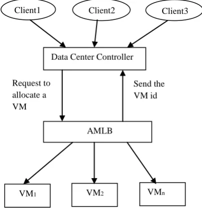
This algorithm is also called as equally spread current execution load balancing. It uses active monitoring load balancer for equally spreading the execution of loads on different virtual machines. The steps of this algorithm are described as follows referring to Fig 1.
Active monitoring load balancer (AMLB) maintains an index table of virtual machines and the number of allocations assigned to each virtual machine. Data Center Controller receives a new request from a client. When a request for allocation of new VM from Data Center Controller arrives at AMLB, it parses the index table from top until the least loaded VM is found. When it finds, it returns the VM id to the Data Center Controller. If there is more than one found, AMLB uses first come first serve (FCFS) basis to choose the least loaded. Simultaneously, it also returns the VM id to the Data Center Controller. Then the Data Center communicates the VM identified by that id. The Data Center Controller notifies the AMLB about the new allocation. After that AMLB updates the allocation table by increasing the allocation count by 1 for that VM. When a VM suitably finishes processing the assigned request, it forwards a response to the Data Center Controller. On receiving the response it notifies the AMLB about the VM de-allocation. The AMLB updates the allocation table by decreasing the allocation count for that VM by 1.
Fig 1. Active monitoring load balancing
3.3
Throttled Load Balancing
This algorithm implements a throttled load balancer (TLB) to monitor the loads on each VM. Here each VM is assigned to only one task at a time and can be assigned another task only when the current task has completed successfully. The algorithm steps can be described as follows:
The job of TLB is to maintain an index table of all VMs as well as their current states (Available or Busy). The client first makes a request to Data Centre Controller for the allocation of appropriate VM and to perform the recommended job. The Data Centre Controller queries the TLB for allocation of the
VM. The TLB scans the index table from top to bottom until the first available VM is found.
If it finds, then TLB returns the VM id to the Data Center Controller. The Data Centre communicates the request to the VM identified by the id. Further, the Data Centre acknowledges TLB about the new allocation and revises the index table by increasing the allocation for that VM by 1.
On the other hand, if the TLB doesn‟t find any VM in the available state it simply returns null. In this case Data Center Controller queues the request until the availability of any VM.
When a VM suitably finishes processing the request, it forwards a response to the Data Center Controller. On receiving it, the Data Center Controller acknowledges the TLB regarding VM de-allocation. The TLB updates the allocation table by decreasing the allocation count for the VM by 1.
In [5] both the authors have proposed a better allocation policy called weighted active monitoring load balancing by assigning weights to each VM.
4.
RESPONSE TIME CALCULATION
The purpose of these algorithms is to calculate the expected response time. We use the following formula for calculation
Response Time = Fint - Arrt + Tdelay
where, Arrt is the arrival time of user request and Fint is the finish time of user request and Tdalay is the transmission delay. However, Tdelay can be calculated as
Tdelay = Tlatency + Ttransfer
Here, Tlatency is the network latency and Ttransfer is the time taken to transfer the size of data of a single request (D) from source location to destination.Tlatency is taken from the latency matrix (after applying Poisson distribution on it for distributing it)held in the internet characteristics.
Ttransfer = D / Bwperuser
where Bwperuser = Bwtotal / N;
Bwtotal is the total available bandwidth (held in the internet characteristics) and N is the number of user requests currently in transmission. The internet characteristics also keep track of the number of user requests in-flight between two regions for the value of N.
5.
SIMULATION
SETUP
AND
COMPARISON OF RESULTS
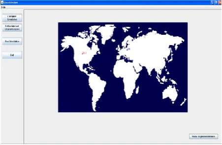
In order to analyze the above discussed algorithms we use the tool called cloud analyst [6]. Basically cloud analyst is a cloudsim [7] based GUI tool used for modelling and analysis of large scale cloud computing environment. Moreover, it enables the modeller to execute the simulation repeatedly with the modifications to the parameters quickly and easily. The following diagram shows the GUI interface of cloud analyst tool.
Client1 Client2 Client3
Data Center Controller
AMLB Request to
allocate a VM
Send the VM id
[image:2.595.53.256.392.601.2]Fig 2. GUI Interface of cloud analyst
It comes with three important menus: configure simulation, define internet characteristics and run simulation [7][8].These menus are used for setting of the entire simulation process. The tool provides us the feature of switching algorithms according to our requirement.
Simulation setup and analysis of results are carried out for a period of 60 hrs by taking different numbers of users, 3 data centers i.e. DC1, DC2, and DC3 having 75, 50 and 25 numbers of VMs respectively. The other parameters are fixed according to Table 1 as shown.
Table 1. Setting of Parameters
Parameter Value Passed
VM-image size 10000
VM-memory 1024 MB
VM-bandwidth 1000
Service broker policy Optimise response time
Data center architecture x86
Data center-OS Linux
Data center-VMM Xen
Data center- No of VMs
DC1-75 DC2-30 DC3-50
Data center-memory per machine 2 GB
Data center-storage per machine 1 TB
Data center-available bandwidth per
machine 1000000
Data center-processor speed 10000
Data center-VM policy Time shared
User grouping factor 1000
Request grouping factor 250
Executable instruction length 250
After performing six different experiments (in short exp) by cloud analyst successfully in two cases we get the overall response time of different load balancing algorithms as given in the Table 2 and Table 4 and overall data center processing time as given in the Table 3 and Table 5.
CASE-1: VMs having Same Number of Processors
In this case we consider all virtual machines having same number of processors i.e. quard core processors.
Table 2. Overall Response Time for Case-1
Setup Description
Overall Response Time (in ms)
Round Robin
Active
Monitoring Throttled
Exp1
6 user bases 187.41 187.52 187.47 Exp2
12 user bases 195.63 195.82 195.67 Exp3
18 user bases 198.19 198.38 198.34 Exp4
24 user bases 199.50 199.56 199.58 Exp5
30 user bases 200.23 200.31 200.27 Exp6
36 user bases 200.87 200.96 200.88 Exp7
42 user bases 201.04 201.11 201.13 Exp8
48 user bases 201.43 201.51 201.44
Table 3. Overall Data Center Processing Time for Case-1
Setup Description
Overall Data Center Processing Time
(in ms)
Round Robin
Active
Monitoring Throttled
Exp1
6 user bases 11.25 11.34 11.37 Exp2
12 user bases 11.35 11.50 11.43 Exp3
18 user bases 11.40 11.48 11.50 Exp4
24 user bases 11.42 11.48 11.50 Exp5
30 user bases 11.43 11.49 11.52 Exp6
36 user bases 11.42 11.51 11.47 Exp7
42 user bases 11.40 11.46 11.48 Exp8
[image:3.595.55.281.72.220.2]CASE-2 VMs having Different Numbers of Processors
[image:4.595.310.551.70.140.2]In this case we consider all virtual machines having different numbers of processors i.e. DC1 having the mixture of dual core and quard core processors, whereas DC2 having only dual core processors and finally DC3 have dual core, quard core and hexa core processors.
Table 4. Overall Response Time for Case-2
Setup Description
Overall Response Time (in ms)
Round Robin
Active
Monitoring Throttled
Exp1
6 user bases 195.91 192.21 192.75
Exp2
12 user bases 200.99 197.28 197.29
Exp3
18 user bases 201.57 199.72 199.14
Exp4
24 user bases 203.69 199.90 199.92
Exp5
30 user bases
204.18 200.45 200.43
Exp6
36 user bases 204.54 200.82 200.84
Exp7
42 user bases 204.79 201.06 201.06
Exp8
[image:4.595.317.544.241.445.2]48 user bases 201.96 201.96 201.28
Table 5. Overall Data Center Processing Time for Case-2
Setup Description
Overall Data Center Processing Time
(in ms)
Round Robin
Active
Monitoring Throttled
Exp1
6 user bases
14.38 10.74 10.72
Exp2
12 user bases 14.39 10.74 10.74
Exp3
18 user bases 14.51 10.79 10.78
Exp4
24 user bases 14.40 10.79 10.78
Exp5
30 user bases 14.37 10.77 10.76
Exp6
36 user bases 14.35 10.78 10.78
Exp7
42 user bases 14.34 10.77 10.77
Exp8
48 user bases 11.42 10.77 11.50
6.
EXPERIMENTAL RESULTS
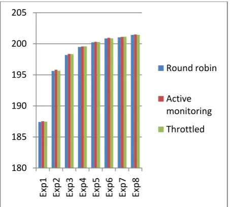
Analytical comparisons of overall response time and overall data center processing time of six different experiments based on various algorithms in cloud computing environment are shown below for two cases. At first case, keeping the number of processor in each VM same we get the following results which are shown in Fig 3 and Fig 4 respectively.
[image:4.595.313.549.468.684.2]Fig 3. Analytical comparison of overall response time for case-1
Fig 4. Analytical comparison of overall data processing time for case-1
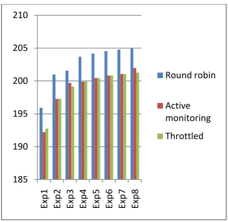
In the second case, we vary the number of processors for each virtual machine and get the overall response time and overall data processing time as shown in the Fig 5 and Fig 6 respectively.
180 185 190 195 200 205
Exp
1
Exp
2
Exp
3
Exp
4
Exp
5
Exp
6
Exp
7
Exp
8
Round robin
Active monitoring
Throttled
11.1 11.15 11.2 11.25 11.3 11.35 11.4 11.45 11.5 11.55
Exp
1
Exp
2
Exp
3
Exp
4
Exp
5
Exp
6
Exp
7
Exp
8
Round robin
Active monitoring
[image:4.595.48.289.501.762.2]Fig 3. Analytical comparison of overall response time for case-2
Fig 4. Analytical comparison of overall data processing time for case-2
7.
CONCLUSION
A greater challenge in minimization of response time is widely seen for each and every engineer of IT sector to develop the products which can increase the efficiency of business performance, customer satisfaction in cloud based environment. Keeping these things in mind we have the endeavour to analyze the three major load balancing algorithms: Round robin, Active monitoring and Throttled. Keeping the number of processors of each VM same we found Round robin load balancing as the efficient one. But practically it may not be possible that each data center has same number of processors per VM. In that case the case-2 is obvious. On the other hand it can help the professionals undoubtedly. We have also found that the parameters: response time, data processing time are almost similar in case of active monitoring and throttled load balancing in both the cases. However, these parameters are slightly improved in case of active monitoring load balancing. Hence we conclude
that active monitoring load balancing is an effective and efficient one than the other two that we have discussed.
8.
ACKNOWLEDGEMENTS
Contribution of many people is a must for the successful completion of any attempt. Our sincere devotion and appreciation to Dr.Gandharb Chandra Nayak, Chairman MGI for his unending support all the way and specially motivating us to develop this research work. We would also like to thank Er. Swapna Kumar Naik, Programmar, Department of CSA, Utkal University for providing us the extensive helping hand at the time of need. Last but not the list, we are grateful to Mr. Abhaya Kumar Jena.
9.
REFERENCES
[1] Rajkumar Buyya, Chee Shin Yeo, Srikumar Venugopal, James Broberg, and Ivona Brandic, “Cloud Computing and Emerging IT Platforms: Vision, Hype, and Reality for Delivering Computing as the 5th Utility, Future Generation Computer Systems”, Volume 25, Number 6, Pages: 599-616, ISSN: 0167-739X, Elsevier Science, Amsterdam, The Netherlands, June 2009.
[2] Ram Prasad Padhy and P Goutam Prasad Rao, “Load balancing in cloud computing systems”, Department of Computer Science and Engineering, National Institute of Technology, Rourkela Rourkela-769008, Orissa, India May, 2011.
[3] Salim Bitam, Abdelhamid Mellouk “ITS-Cloud: Cloud Computing for Intelligent Transportation System”, Globecom 2012- Communications Software, Services and Multimedia Symposium.
[4] Saroj Hiranwal and Dr. K.C. Roy, “Adaptive Round Robin Scheduling Using Shortest Burst Approach Based On Smart Time Slice” International Journal Of Computer Science And Communication July-December 2011 ,Vol. 2, No. 2 , Pp. 319-323.
[5] Jasmin James and Dr. Bhupendra Verma, “Efficient VM load balancing algorithm for a cloud computing environment”, International Journal on Computer Science and Engineering (IJCSE), 09 Sep 2012.
[6] Bhathiya Wickremasinghe, “CloudAnalyst: A CloudSim based Tool for Modelling and Analysis of Large Scale Cloud Computing Environments” MEDC project report, 433-659 Distributed Computing project, CSSE department., University of Melbourne, 2009.
[7] R. Buyya, R. Ranjan, and R. N. Calheiros, “Modeling And Simulation Of Scalable Cloud Computing Environments And The Cloudsim Toolkit: Challenges And Opportunities,” Proc. Of The 7th High Performance Computing And Simulation Conference (HPCS 09), IEEE Computer Society, June 2009.
[8] Judith Hurwitz, Robin Bloor, and Marcia Kaufman, “Cloud computing for dummies” Wiley Publication (2010).
185 190 195 200 205 210
Exp
1
Exp
2
Exp
3
Exp
4
Exp
5
Exp
6
Exp
7
Exp
8
Round robin
Active monitoring
Throttled
0 2 4 6 8 10 12 14 16
Exp
1
Exp
2
Exp
3
Exp
4
Exp
5
Exp
6
Exp
7
Exp
8
Round robin
Active monitoring
10.
AUTHORS’ PROFILE
Er. Soumya Ranjan Jena, B.Tech in CSE (from BPUT), CCNA (from CTTC), M.Tech in Information Technology (from Utkal University) is presently working as Asst. Professor, Department of Computer Science and Engineering, M.I.E.T, Bhubaneswar, Odisha, India. He has authored a book on “Design and Analysis of Algorithms” published by Kalyani Publishers, New Delhi, India. His
special fields of interest include cloud computing, computer networking, cyber security, algorithms, and theory of computation.