A Neuro fuzzy Computing Technique for Modeling the Acoustic Form Function of Immersed Tubes

A Neuro-Fuzzy Computing Technique for

Modeling the Acoustic Form Function of

Immersed Tubes

Y.Nahraoui

LMTI, Faculté des sciences,

Université Ibn Zohr, Agadir, Maroc

EL H.Aassif

LMTI, Faculté des sciences,

Université Ibn Zohr, Agadir, Maroc

G.Maze

LOMC, Laboratoire des Ondes et Milieux Complexes FRE

CNRS 3201, Université du Havre,

Le Havre, France

A.Elhanaoui

LMTI, Faculté des sciences,

Université Ibn Zohr, Agadir, Maroc

ABSTRACT

An Adaptative Neuro-Fuzzy Inference System (ANFIS) is developed to predict the acoustic form function (FF) for an infinite length cylindrical shell excited perpendicularly to its axis. The Wigner-Ville distribution (WVD) is used like a comparison tool between the calculated FF by the analytical method and that predicted by the neuro-fuzzy technique for a copper tube. During the application of this technique, several configurations are evaluated for various radius ratio b/a (a: outer radius, b: inner radius of tube). This neuro-fuzzy technique is able to predict the FF with a mean relative error (MRE) about 1.7%.

Keywords

—ANFIS, acoustic scattering, cylindrical shells, Wigner-Ville distribution.

1.

INTRODUCTION

Many studies, theoretical and experimental, show that acoustic resonances of a target are related to its physical and geometrical properties. Conversely, starting from these resonances, we can characterize the material constituting a target with a known geometry. Among all the targets of simple geometrical forms (plate, cylinder, sphere, tube...), tubes are the subject of few studies of characterization[1-12]. If an air-filled tube immersed in water is excited by a plane acoustic wave perpendicularly to its axis, circumferential waves are generated in the shell and in the water/shell interface [13,14]. For some frequencies, these circumferential waves form stationary waves on the circumference of the tube constituting resonances [14]. The mode n of a resonance is the number of wavelengths around the circumference. These resonances are observed on the spectrum of the acoustic pressure backscattered (or the form function) by the tube [3, 5]. The circumferential waves can belong to two wave types which are equivalent to the Lamb waves on a plate if the shell wall is thin: the anti-symmetric (Ai) and symmetric (Si)

circumferential waves (i = 0, 1, 2, …: index of wave)[5,9,13].

For a tube made of a given material, the reduced resonance frequencies of these waves essentially depend on the radius ratio b/a [6, 8]. The resonance modes n of a surface wave line up on trajectories (n as function of the reduced frequency called Regge trajectories)[5,15]. For i 1, these trajectories have reduced cut-off frequencies, which depend on the physical characteristics of the tube[16]. The aim of this paper is to compare the form function predicted by ANFIS techniques with that obtained analytically. The Wigner-Ville time-frequency distribution was used as a comparison tool to check the validity of the use of the ANFIS network model to predict the form function [16]. The analysis of this time-frequency distribution takes into account both the time parameter and the frequency parameter leading to synthetic images that allow us to follow the evolution of the frequential content of a wave echo as a time function [17, 18]. Major benefits using ANFIS network are excellent management of uncertainties, noisy data and non-linear relationships. In this study, the ANFIS model predicts the form functions of tubes without the use of the analytical method for various radius ratio b/a. For each b/a, the input training data for ANFIS is a four-dimensional vector of the following form. w(t) = [FF(t-4) FF(t-3) FF(t-2) FF(t-1)].

The output training data corresponds to the trajectory prediction. s(t) = F(t). This model is able to predict the FF for copper tube of various radius ratio b/a between 0.9 and 0.99.

2. BACKSCATTERED ACOUSTIC

SIGNAL FROM A TUBE

The acoustic plane wave with frequency ɷ insonifies the cylindrical shell normally to the z-axis. The fluid 2 filling the cavity of the shell has a density 2 and the velocity of

longitudinal wave in this fluid is c2. In general, the outer fluid,

labelled fluid 1, is different and its density is 1 and the

velocity of wave is c1.

In this study, an air-filled tube immersed in water is excited by a plane acoustic wave perpendicularly to its axis (Fig.1). The complex pressure

P

_scat



backscattered by the tube in a far field is the sum of the normal modes which takes into account the effects of the incident wave, the reflective wave {1}, surface waves in the shell {2} (whispering gallery waves, Rayleigh wave: equivalent to Lamb waves if the tube wall is thin) and an antisymmetrical interface Scholte A wave labelled also A0 wave{3} connected to the geometry of the

object (Fig.2) [22]. Waves {2} and {3} are the circumferential waves. In our case, the flexural waves A, A1 and A2 and the

[image:2.595.322.544.303.427.2]

compression waves S0, S1 and S2 can be observed.

Fig. 1. The geometry used to calculate the form function for an elastic tube.

Fig. 2. Mechanisms of the echo formation ({1}: specular

reflection, {2}: circumferential shell

The general analytical form of the backscattered pressure

scat

P



in far field at normal incidence can be expressed as:

1

0 1

0 1

( )

1

( )

exp (

)

cos(

).

( )

n

scat n

n n

D

i

P

P

i k r

t

n

D

k r















 











(1)

where  is the angular frequency, k1 is the wave-number with

respect to the wave velocity in the external fluid, P0 is the

amplitude of the incident plane wave, r is the distance of pressure measurement, Ɵ is the azimuthal angle (Ɵ = 180° for the backscattering spectrum), Dn1() and Dn() are

determinants computed from the boundary conditions of the problem (continuity of stress and displacement of both interfaces), the terms of these determinants are given in ref 7 (in the present study, the normal incidence is only considered) and εn is the Neumann coefficient (εn =1 if n=0 and εn =2 if

n0).

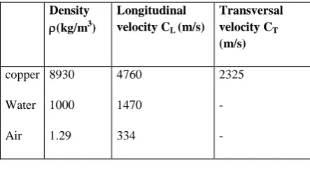
The physical parameters used in the calculation of the backscattered complex pressure are illustrated in Table I.

Table 1. Physical parametrs

Usually this backscattered pressure is presented as the form function FF defined by the relation (2)[23]:

scat

0

P

a

FF

P

2r





(2)

This form function is function of the reduced frequency x1=k1a given by:

1

1

2

a

k a

c





(3)

where

2









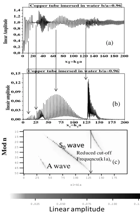
is the frequency of a wave in Hz.

Figs. 3 shows an example of results computed for a copper tube (b/a = 0.96). The backscattered pressure spectrum is presented on Fig. 3(a). It is obtained from the computation of the form function FF (2). From the backscattered complex pressure, the impulse time response is calculated with an inverse Fourier transform (4), the function h(ɷ) is the bandpass of transducers used in the experiments.

1

( )

( )

( )

2

i t

scat

scat

P

t

h



P



e



d



















(4)

Density

(kg/m3₎

Longitudinal velocity CL (m/s)

Transversal velocity CT

(m/s)

copper 8930 4760 2325

Water 1000 1470 -

[image:2.595.58.279.327.643.2]

Examples of results are given in refs. 6 and 22. To obtain a resonance spectrum using “Resonance Scattering Theory” (RST), the theoretical studies indicate that it is possible to suppress the rigid background for the thick cylindrical shells, the soft background for the very thin shell and intermediate background for the other tubes. [2, 3, 25] It is possible to obtain the resonance spectrum using another method developed in first time in experiment and applied to theoretical results: a new Fourier transform is applied to the impulse time signal in which the specular echo (reflected echo) is suppressed and replaced by zeroes, this technique supresses the real background and the obtained spectrum is the backscattered resonance spectrum presented on Fig. 3(b) [26]. The amplitude transitions (Fig. 3(a)) are related to the peaks observed (arrows) on Fig. 3(b) [2, 3, 25]. These peaks are due to the resonances of modes n, they are connected with the propagation of circumferential waves [3, 13, 27]. When a circumferential wave is generated on the shell, a resonance establishes when the number of wavelengths on the circumference of the tube is an integer, this integer is the mode n. To plot the figure 3(c), the resonance spectra are calculated for each values of n with the previously technique and associated in a plane “n-k1a” with amplitude in grey

level. The trajectories of the modes n of resonances in the same frequency domain (0<x1<200) are Regge trajectories [5,

15]. Each trajectory is related to a wave type (A, S0, A1). The

trajectory in relation to the A1 wave has a cut-off frequency

for the small values of the mode n indicated by an arrow on Figure 3(c).

3. WIGNER-VILLE TIME FREQUENCY

DISTRIBUTION

The Wigner-Ville Distribution (WVD) presents some convenient properties of applications such as energy conservation, time and frequency shift invariance and preservation of the time duration and bandwidth [18]. The time-frequency analysis takes into account both the time parameter and the frequency parameter leading to an image that allows us to follow the evolution of the frequency content of acoustic echoes as a function of time [28].

Among the time-frequency techniques, WVD is used for its interesting properties in terms of acoustic applications [16]. Other time-frequency methods (wavelets for example) would be used in our application but we had good results with the WVD [17]. The WVD is applied to obtain the dispersion curves of the group and phase velocities of circumferential waves propagating around a tube with different radius ratio [16]. The WVD can be applied to the backscattered time signal obtained from the computation and/or the experiment. This allows us to determine the reduced cut-off frequencies [16].

The WVD of time complex signal u(t) displays the energy distribution of this signal in the time-frequency plane (5).

0 20 40 60 80 100 120 140 160 180 200 0,0

0,2 0,4 0,6 0,8 1,0 1,2 1,4

lin

ea

r A

m

pl

itu

de

x1=k1a

Copper tube imersed in water b/a=0.96

0 25 50 75 100 125 150 175 200 0,00

0,03 0,06 0,09 0,12 0,15

lin

ea

ir

am

pl

itu

de

x1=k1a

Copper tube imersed in water b/a=0.96

0 25 50 75 100 125 150 175

10

15 20

25 30

35

40 45

50

x1=k1a

Mode n

0.025 0.050 0.075 0.100 0.125

spec_res_n_cu_96_ddc_s_x_x

Linear amplitude

Reduced cut-off

Frequencu(k1a)c

A wave

S

₀

wave

(a)

(

b)

(c)

M

o

d

n

Fig. 3 Form function spectrum, (b) Resonance spectrum and (c) Trajectories of modes n for an air-filled copper cylindrical shell (b/a=0.96) immersed in water. Arrows indicate the relation between transition (a) and peak (b). The reduced cut-off frequency of the A1 wave is indicate

by a vertical line (c).

( , )

(

) *(

) exp ( 2

)

2

2

u

W t





u t



u

t



i

   

d





_







(5)

with

2









the frequency and t the time of the signal,

u*(t) is the conjugated complex time signal of u(t).

4. NEURO-FUZZY MODEL

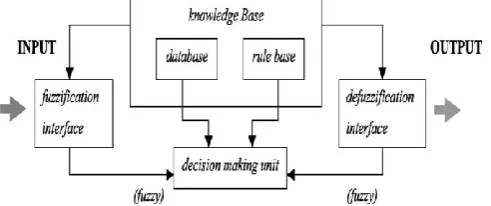
The basic structure of a FIS consists of three conceptual components: a rule base, which contains a selection of fuzzy rules; a database which defines the membership functions (MF) used in the fuzzy rules; and a reasoning mechanism, which performs the inference procedure the rules to derive an output (see Fig. 4). FIS implements a nonlinear mapping from its input space to the output space.

[image:3.595.320.565.86.460.2]

specifically, the configuration of an adaptive network is composed of a set of nodes connected through directional links, where each node is a process unit that performs a static node function on its incoming signal to generate a single node output. The node function is a parameterized function with modifiable parameters. It may be noted that links in an adaptive network only indicate the flow direction of signals between nodes and no weights are associated with these links. Readers are referred to [19] for more details on adaptive networks. Jang [20] introduced a novel architecture and learning procedure for the FIS that uses a neural network learning algorithm for constructing a set of fuzzy if-then rules with appropriate MFs from the stipulated input–output pairs. This procedure of developing a FIS using the framework of adaptive neural networks is called an adaptive neuro fuzzy inference system (ANFIS).

[image:4.595.54.300.251.354.2]

Fig. 4. Fuzzy Inference System with crisp output.

4.1 ANFIS Architecture

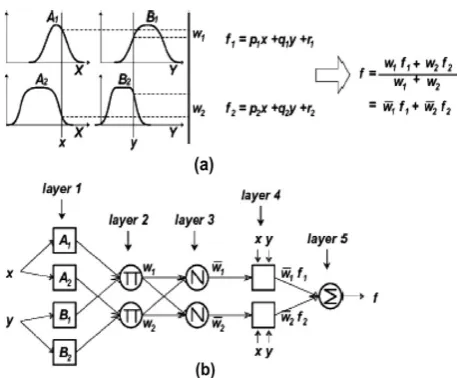
The general structure of the ANFIS is presented in Fig. 5(b). Selection of the FIS is the major concern when designing an ANFIS to model a specific target system. Various types of FIS are reported in the literature (e.g. [21]; [23]; [29] and each are characterized by their consequent parameters only. The current study uses the Sugeno fuzzy model [29]; [30] since the consequent part of this FIS is a linear equation and the parameters can be estimated by combination of the gradient descent method and the least squares estimate (LSE), for this study we consider that the FIS has two inputs x and y and one output f: For the first order Sugenofuzzy model, a typical rule set with two fuzzy if-thenrules can be expressed as:

Rule 1: If x is A1 and y is B1, then f1=p1 x+q1 y+r1 (6)

Rule 2: If x is A2 and y is B2, then f2=p2 x+q2 y+r2 (7)

where A1; A2 and B1; B2 are the MFs for inputs x and y; respectively; p1; q1; r1 and p2; q2; r2 are the parameters of the output function. Fig. 5(a)illustrates the fuzzy reasoning mechanism for this Sugeno model to derive an output function (f) from a given input vector [x, y].

The corresponding equivalent ANFIS architecture is presented in Fig.5(b), where nodes of the same layer have similar functions. The functioning of the ANFIS is as follows:

Layer 1: Each node in this layer generates membership grades of an input variable. The node output

OP

₁iis defined by:

1 _i

( )

i A

OP





x

for i=1,2 or

(8)

2

1 _i

( )

i B

OP





_

x

for i=3,4

where x (or y) is the input to the node; Ai (or Bi-2) is a fuzzy set associated with this node, characterized by the shape of the MFs in this node and can be any appropriate functions that are continuous and piecewise differentiable such as generalized bell shaped functions. Assuming a generalized bell function as the MF, the output

OP

₁i can be computed as,

1

2

1

( )

1 (

)

i

i i

A

b i

i

OP

x

x c

a







_



(9)

where {ai; bi; ci} is the parameter set that changes the shapes

of the MF with maximum equal to 1 and minimum equal to 0.

Layer 2: Every node in this layer multiplies the incoming signals, denoted as



, and the output

OP

_i2that represents the firing strength of a rule is computed as,

2

( )

( ),

1, 2.

i i

i i A B

OP



 



x



y i



(10)

Layer 3: The ith node of this layer, labeled as N; computes the normalized firing strengths as,

3

1 2

,

1, 2.

i

i i

OP





i

 









(11) Layer 4: Node i in this layer computes the contribution of the ith rule towards the model output, with the following node function:

OP

_i4





_i

f

_i





_i

(

p x q x r

_i



_i



_i

)

(12) where



is the output of layer 3 and {pi; qi; ri} is the parameter set

Layer 5: The single node in this layer computes the overall output of the ANFIS as:

5 1

i i i i i i

i i

f

OP

Overall output

f



















(13)

4.2 Estimation of Parameters

Fig.5. (a) First-order Sugeno fuzzy model, (b) ANFIS architecture

and the consequent parameters {pi; qi; ri}; which describe the overall output of the system. The basic learning rule of an adaptive network is based on combination of the gradient descent method and the least squares estimate (LSE) to identify parameters.

From the ANFIS architecture presented in Fig. 5 it is observed that given the values of the premise parameters, the overall output can be expressed as linear combinations of consequent parameters. More precisely, the output f can be rewritten as:

1 1 2 2

1 1 1 1 1 2 2 2 2 2 2

(

)

(

)

( )

(

)

(

)

(

)

f

f

f

x p

y q

r

x p

y q

r

































(14) which is linear in the consequent parameters (p1; q1; r1; p2; q2 and r2). As a result, the total number of parameters S in an ANFIS can be divided into two such that S1 = set of premise parameters and S2= set of consequent parameters. Consequently the hybridlearning algorithm, which combines the backpropagation gradient descent and least squares method, can be used for an effective search of the optimal parameters of the ANFIS. More specifically, in the forward pass of the hybrid learning algorithm, the node output goes forward until layer 4 and the consequent parameters are identified by the least squares method. In the backward pass, the error signal propagates backwards and the premise parameters are updated by gradient descent. As mentioned earlier, the consequent parameters thus identified are optimal under the condition that the premise parameters are fixed. Accordingly, the hybrid approach converges much faster since it reduces the dimension of the search space of the original back-propagation method. A detailed description of this algorithm can be found in [31].

5.

APPLICATION

OF

THE

ADAPTATIVE

NEURO-FUZZY

INFERENCE

SYSTEM

(ANFIS)

NETWORKS TO PREDICT FF

System modelling based on conventional mathematical tools (eg., differential equations) is not well suited for dealing with ill-defined and uncertain systems. By contrast, an ANFIS modelling employing fuzzy if-then rules can model the qualitative aspects of human knowledge and raisoning processes without employing precise quantitative analyses. The advantage of ANFIS networks is that they are capables of a linear and nonlinear modelling of systems.

In the present study, we use an ANFIS trained with the gradient descent (jang 91) backpropagation and last squares algorithm to achieve the learning ability to predict the form function for a copper tubes [31, 32].

ANFIS method constitutes a new approach of prediction of the form function for various radius ratio b/a of tubes included in the interval [0.4-0.99]. With this method we can also find easily to the radius ration b/a of an unknown form function for a tube of material given.

5.1 ANFIS Model and Training Phase

ANFIS networks method requires for its training a set of form functions calculated by the analytical method or obtained by experiments.

In this work, the dataset is constituted from the form functions calculated by the analytical method. This dataset is divided into two sets. The first 1000 training data set was used for training the ANFIS while the remaining 1000 checking data set were used for validating the identified model, the number of membership function is fixed to 2 MF, so the rule number is 16 . The ANFIS used here contains a total of 104 fitting parameters, of which 24 are premise parameters and 80 are consequent parameters. The desired and predicted values for both training data and checking data are essentially the same in fig 7, 8 and 9 and their difference. The input vector of the ANFIS is represented by the radius ratio b/a and the FF values for the preceding four indexes of dimensionless frequency

1 1 1

1 1

( )

( 1)

(

2)

(

3)

(

4)

(

)

[ ,(

)

,(

)

,

(

)

,(

)

,]

x i

x i

x i

x i

x i

b

FF

ANFIS

FF

FF

a

FF

FF











(15) Once the dataset is constructed, it remains to train the NAFIS using the combination of last square error and the back-propagation gradient descent algorithm to predict the form function.

[image:5.595.52.281.67.256.2]

5.2 Selection of the Optimal Model

The performance of ANFIS models for training and testing data sets were evaluated according to statistical criteria such as, coefficient of correlation R, MAE, MRE, SE, and root mean square error (RMSE). The selection of different models is done comparing the errors of the ANFIS configuration, calculating the MAE, the MRE and the SE of the cut-off frequency. The coefficient of correlation R and the determination R2 _{of the linear regression are used like}

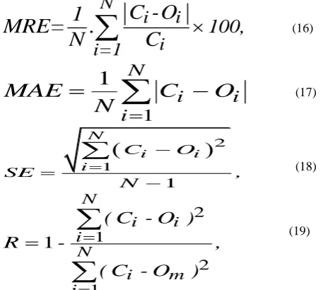
performance measures of the model between the predicated and the desired output. The different error measures and the coefficient of correlation are given by the following relations:

N

i

i

i

i=1

100,

C -O

1

MRE=

.

N



C



(16)

1

1

N

i

i

i

MAE

C

O

N

_







(17)





2

1

1

N

i i

i

C O

SE ,

N



 





(18)

2

1

2

1

1

N

i

i

i

N

i

m

i

( C - O )

R

-

,

( C - O

)











(19)

where N is the number of data, Ci and Oi are respectively the

desired and the predicted values. Om is the mean of the

predicted values.

6. RESULTS AND DISCUSSION

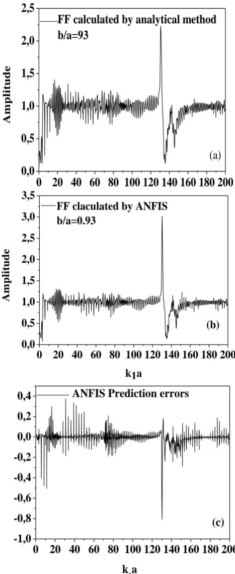
The ANFIS is trained by using randomly 50% of the dataset. While the remaining dataset 50% is reserved as a test base. The analysis is repeated several times. Indeed, the values of errors are measured for ANFIS network architecture. The best configuration is found for a network with the number of membership function is fixed to 2 MF, so the rule number is 16. The MRE and the SE for the optimal model are respectively 1.9% and 6.10-4 k1a for b/a=0.97 (Fig.6). Figures 7, 8, 9 and 10 show the comparison between the form functions predicted by the ANFIS model on a test database and that calculated by the analytical method for the radius ratios b/a = 0.93, 0.95 and 0.97. Figures 7, 8 and 9) shows the good agreement between the predicted and the calculated values of the form function.

Table III. Comparison between the reduced cut-off frequencies computed by eigen modes method and starting from the Wigner-Ville image

Circumferential wave A1

(k1a)c Estimated

(WV) by analytical method

(k1a)c Estimated

(WV) by ANFIS

b/a=0.93 70.94±0.3 70.48±0.3

b/a=0.95 99.32±0.3 99.94.0±0.3

b/a=0.97 165.54±0.2 165.00±0.2

0,0

0,5

1,0

1,5

2,0

0,0

0,5

1,0

1,5

2,0

2,5

3,0

P

r

e

d

ic

te

d

F

o

r

m

F

u

n

c

ti

o

n

calculated Function Form

on a test base

ANFIS with 16 Rules

b/a=0.93

R=0.93

MRE=1.9%

MAE=1.7%

SE=8.10

-3

(a)

0,0

0,5

1,0

1,5

2,0

2,5

0,0

0,5

1,0

1,5

2,0

2,5

3,0

3,5

P

r

e

d

ic

te

d

f

o

r

m

f

u

n

c

ti

o

n

Calculated form function

on a test base

ANFIS with 16 Rules

b/a=0.95

R=0.94

MRE=3.2%

MAE=2.7%

SE=1.5.10

-3

(b)

0,0

0,2

0,4

0,6

0,8

1,0

1,2

1,4

0,0

0,2

0,4

0,6

0,8

1,0

1,2

1,4

P

r

e

d

ic

te

d

f

o

r

m

f

u

n

c

ti

o

n

Calculated form function

on a test base

ANFIS with 16 Rules

b/a=0.97

R=0.93

MRE=1.9%

MAE=1.7%

SE=6.10

-4

(c)

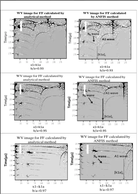
[image:6.595.312.550.62.715.2] [image:6.595.54.283.205.410.2]

However, the time-frequency representation of Wigner-Ville is used as a tool of comparison to check the validity of the ANFIS network model because the studied signals are not stationary. Using a time-frequency representation can allow us to follow the evolution of the frequency content of acoustic echoes as a function of time. Figure 10 shows the good

0

20 40 60 80 100 120 140 160 180 200

0,0

0,5

1,0

1,5

2,0

2,5

3,0

3,5

A

m

p

li

tu

d

e

k1a

FF claculated by ANFIS

b/a=0.93

(b)

0

20 40 60 80 100 120 140 160 180 200

-1,0

-0,8

-0,6

-0,4

-0,2

0,0

0,2

0,4

k

₁

a

ANFIS Prediction errors

(c)

0 20 40 60 80 100 120 140 160 180 200

0,0

0,5

1,0

1,5

2,0

2,5

A

m

p

li

tu

d

e

FF calculated by analytical method

b/a=93

[image:7.595.314.554.100.628.2]

(a)

Fig 7: Form Function calculated by analytical methodand form Function predicted by ANFIS for b/a=0.93

agreement between Wigner-Ville image of the predicted and

the calculated form function for a copper tube of radius ratio b/a=0.93, 0.95 and 0.97. Moreover, starting from the Wigner-Ville image of the predicted signal, the reduced cut-off frequency ([k1a]c) of the tube corresponding to the A1 wave

can be determined. Generally, the ANFIS networks methods

0 20 40 60 80 100 120 140 160 180 200 0,0

0,5 1,0 1,5 2,0 2,5

A

m

p

li

tu

d

e

FF calculated by analytical method b/a=0.95

(a)

0

20 40 60 80 100 120 140 160 180 200

0,0

0,5

1,0

1,5

2,0

2,5

3,0

3,5

A

m

p

li

tu

d

e

k1a

FF claulated by ANFIS

b/a=0.95

(b)

0 20 40 60 80 100 120 140 160 180 200 -1,0

-0,8 -0,6 -0,4 -0,2 0,0 0,2 0,4 0,6

k1a

ANFIS prediction errors

[image:7.595.54.288.145.716.2]

(c)

Fig 8: Form Function calculated by analytical method and form Function predicted by ANFIS for b/a=0.95

The circumferential antisymmetric A1 waves propagates

around the circumference of the tube only for frequencies superior to the reduced cut-off frequency [31]. The reduced cut-off frequency values ([k1a])c) obtained from the Wigner-

0

20 40 60 80 100 120 140 160 180 200

0,0

0,2

0,4

0,6

0,8

1,0

1,2

1,4

A

m

p

li

tu

d

e

FF calculated by analytical methode

b/a=0.97

(a)

0

20 40 60 80 100 120 140 160 180 200

0,0

0,5

1,0

1,5

A

m

p

li

tu

d

e

k1a

FF calculated by ANFIS

b/a=0.97

(b)

0

20 40 60 80 100 120 140 160 180 200

-0,6

-0,5

-0,4

-0,3

-0,2

-0,1

0,0

0,1

0,2

0,3

0,4

k

₁

a

ANFIS prediction errors

(c)

Fig 9: Form function calculated by analytical methodand form Function predicted by ANFIS for b/a=0.97

Ville image of the test database (b/a=0.93, 0.95, 0.97) and analytically calculated are presented in Table III.

Starting from the operating mode direction of this optimal model we can make several things. In direct operating mode of the model optimal, one can predict the form functions for tubes of various radius ratio b/a and for various materials.

6. CONCLUSION

This paper presents the application of an ANFIS model to predict the form function for a copper tube. We can say that the results obtained with the new proposed approach have been good and positive in predicting. This model is able to

T

im

e(µ

s)

25 50 75 100 125 150 175 25 50 75 100 125 150 175 col row

-5.0e-007 -2.5e-007 0.0e+000 2.5e-007 5.0e-007 7.5e-007 wv93th_txt_s_x

25 50 75 100 125 150 175 25 50 75 100 125 150 175 col row

-2.50e-0070.00e+000 2.50e-007 5.00e-007 7.50e-007 1.00e-006 1.25e-006 FLwv_txt_s_x_x

WV image for FF calculated by analytical method

WV image for FF calculated by ANFIS method

x1=k1a b/a=0.93 Ti m e( µs ) x1=k1a b/a=0.93 A1 wave [k1a]c

S0wave

25 50 75 100 125 150 175 25 50 75 100 125 150 175 col row

-4e-007 -2e-007 0e+000 2e-007 4e-007 6e-007 wvth_txt_s_x

25 50 75 100 125 150 175 25 50 75 100 125 150 175 col row

-7.50e-007-5.00e-007-2.50e-007-5.68e-0142.50e-0075.00e-0077.50e-0071.00e-0061.25e-006 wv95FL_txt_s_x

WV image for FF calculated by

analytical method WV image for FF calculated by _{ANFIS method}

Ti m e( µs ) Ti m e( µs ) x1=k1a b/a=0.95 x1=k1a b/a=0.95 A1 wave [k1a]c

S0wave

WV image for FF calculated by ANFIS method

25 50 75 100 125 150 175 25 50 75 100 125 150 175 col row

-1.25e-0070.00e+000 1.25e-007 2.50e-007 3.75e-0075.00e-007 6.25e-007 wv97th_txt_s_x

25 50 75 100 125 150 175 25 50 75 100 125 150 175 col row

-2.50e-007 -1.25e-007 0.00e+000 1.25e-007 2.50e-007 3.75e-007 5.00e-007 wv97FL_txt_s_x_x

[image:8.595.57.295.131.638.2] [image:8.595.316.556.166.504.2]

WV image for FF calculated by analytical method x1=k1a b/a=0.97 x1=k1a b/a=0.97 Ti m e( µ s) Ti m e( µ s) [k1a]c A1 wave S0wave

Fig. 10. Comparison between the WV images for the form function calculated by the analytical method and predicted by the ANFIS method (b/a=0.93, 0.95 and 0.97).

predict the FF with a Mean Relative Error (MRE) about 1.9%. In this article, the ANFIS approach can be used as a new tool for non-destructive characterization of a thin elastic tube. To check the credibility of the ANFIS model in the time and frequency domains, time-frequency representation of Wigner-Ville was used like tool of comparison between the FF calculated by the analytical method and that predicted by the ANFIS technique.

7. REFERENCES

[1] Hickling R., Analysis of echoes from a hollow metallic sphere in water, J.coust Soc. Am. 36, 1124-1137 (1964). [2] Flax L., Dragonette L.R., Überall H., Theory of elastic

resonance excitation by sound scattering, J. Acoust Soc. Am. 63, 723-731 (1978).

[3] Murphy J.D., Breitenbach E.D., Überall H., Resonance scattering of acoustic waves from cylindrical shells, J. Acoust Soc. Am. 64, 677-683 (1978).

[4] Maze G., Ripoche J ., Visualization of acoustic scattering by elastic cylinders at low ka, J. Acoust Soc. Am. 73, 41-43 (1983).

[5] Maze G., Izbicki J.-L., Ripoche J., Resonances of plates and cylinders: Guided waves, J. Acoust Soc. Am. 77, 1352-1357 (1985).

[6] Maze G., Acoustic scattering from submerged cylinders, MIIR Im/Re: Experimental and theoretical study, J. Acoust Soc. Am. 89, 2559-2566 (1991).

[7] Léon F., Lecroq F., Décultot D., Maze G., Scattering of an obliquely incident acoustic wave by an infinite hollow cylindrical shell, J. Acoust Soc. Am. 91, 1388-1397 (1992).

[8] Ripoche J., Maze G., A new acoustic spectroscopy: The resonance scattering spectroscopy by the MIIR, “Acoustic Resonance Scattering”, Redactor H. Überall, Editor Gordon and Breach, New York, 1992, (ISBN 2-88124-513-7), § 5, 69-103.

[9] Décultot D., Lecroq F., Maze G., Ripoche J., Acoustic scattering from a cylindrical shell bounded by hemispherical endcaps. Resonance explanation with surface waves propagating in cylindrical and spherical shells, J. Acoust Soc. Am. 94, 2916-2923 (1993). [10] Veksler N., Maze G., Ripoche J., Porochovskii V.,

Scattering of obliquely incident plane acoustic wave by circular cylindrical shell. Results of computations., Acta Acustica 82, 689-697 (1996) and Maze G., Léon F., Veksler N., Scattering of an obliquely incident plane acoustic wave by circular cylindrical shell. Experimental results, Acta Acustica 84, 1-11 (1997).

[11] Morse S.F., Marston P.L., Kaduchak G., High-frequency backscattering enhancements by thick finite cylindrical shells in water at oblique incidence: Experiments, interpretation and calculations, J. Acoust Soc. Am. 103, 785-794 (1998).

[12] Haumesser L., Décultot D., Léon F., Maze G., Acoustic scattering from a finite cylindrical shell at oblique incidence : Experimental identification along the shell length, J. Acoust Soc. Am. 111, 2034-2039 (2002). [13] Talmant M, Quentin G, Rousselot JL, Subrahmanyam

JV, and Überall H. Acoustic resonances of thin cylindrical shells and the resonance scattering theory. J. Acoust. Soc. Am. 84, 681-688 (1988).

[14] Frisk G.V., Dickey J.W., Überall H., Surface wave modes on elastic cylinders, J. Acoust Soc. Am. 58, 996-1008 (1975).

[15] Izbicki J.L., Maze G., Ripoche J., Influence of the free modes of vibration on the acoustic scattering of a circular cylindrical shell, J. Acoust Soc. Am. 80, 1215-1219 (1986).

[16] Latif R., Aassif E.H., Maze G; Décultot D., Moudden Ali, Determination of group and phase velocities from time-frequency representation of Wigner-Ville, NDT & E International 32, 415-422 (1999) and Latif R., Aassif E.H., Moudden A., Décultot D., Faiz B., Maze G; Determination of the cutoff frequency of an acoustic circumferential wave using a time-frequency analysis, NDT & E International 33, 373-376 (2000).

[17] Yen N, Dragonette L, K. Numrich S. Time-frequency analysis of acoustic scattering from elastic objects. J. Acoust. Soc. Am. 87, 2359-2370 (1990).

[18] Claasen TACM, Mecklenbrauker WFG. The Wigner-Distribution tools for time-frequency signal analysis. Philips J. Res. Vol. 35, n° 3, 4, 5, 217-250, 276-300 and 372-389 (1980).

[19] Brown, M., Harris, C., 1994. Neurofuzzy Adaptive Modeling and Control. Prentice Hall.

[20] Jang, J.-S.R., 1993. ANFIS: adaptive network based fuzzy inference system. IEEE Transactions on Systems, Man and Cybernetics 23 (3), 665–683.

[21] Mamdani, E.H., Assilian, S., 1975. An experiment in linguistic synthesis with a fuzzy logic controller. International Journal of Man-Machine Studies 7 (1), 1– 13.

[22] Maze G., Léon F., Ripoche J., and Überall H. Repulsion phenomena in the phase-velocity dispersion curves of circumferential waves on elastic cylindrical shells, J. Acoust. Soc. Amer. 105, 1695-1701 (1999) and Maze G., Touraine N., Baillard A., Décultot D., Latard V, Derbesse L., Pernod P., Merlen A., A0-wave and A-wave in cylindrical shell immersed in water: influence on the acoustic scattering, (1999) ASME, DECT, Las Vegas, Nevada, USA 12-16 sept 1999, Proceeding on CD-Rom. [23] Flax L., Neubauer W. G., Acoustic reflection from

layered elastic absorptive cylinders,J. Acoust. Soc. Am. 61, 307-312 (1977).

[24] Tsukamoto, Y., 1979. An approach to fuzzy reasoning method. In: Gupta, M.M., Ragade, R.K., Yager, R.R. (Eds.), Advances in Fuzzy Set Theory and Application, North-Holland, Amsterdam, pp. 137–149.

[25] Veksler N., Resonance Acoustic Spectroscopy, Springer Series on Wave Phenomena, Springer-Verlag, (1993)Berlin, Heidelberg, New York, ISBN 3-540-55638-9.

[26] Pareige P., Rembert P, Izbicki J.-L., Maze G., Ripoche J., Méthode impulsionnelle numérisée (MIN) pour l’isolement et l’identification des résonances de tubes immergés, (digital impulse method for isolation and identification of resonances of immersed tubes), Physics Letters 135A, 143-146 (1989).

[27] Sun N. H., Marston P. L., Ray synthesis of leaky Lamb wave contributions to backscattering from thick cylindrical shells, J. Acoust. Soc. Amer. 91, 1398-1402 (1992).

[28] Hughes DH, Marston PL. Local temporal variance of Wigner’s distribution function as a spectroscopic observable: Lamb wave resonances of a spherical shell. J. Acoust. Soc. Amer. 94, 499-505 (1993).

[29] Takagi, T., Sugeno, M., 1985. Fuzzy identification of systems and its application to modeling and control. IEEE Transactions onSystems, Man and Cybernetics 15 (1), 116–132.

[30] Sugeno, M., Kang, G.T., 1988. Structure identification of fuzzy model. Fuzzy Sets and Systems 28, 15–33. [31] Jang, J.-S.R., 1991. Rule extraction using generalized

neural networks. In Proceedings of the fourth IFSA World Congress 4, 82–86.Volume for Artificial Intelligence.