An Algorithm for Traffic Equilibrium Flow with Capacity Constraints of Arcs

(1)

http://dx.doi.org/10.4236/jtts.2015.54022

An Algorithm for Traffic Equilibrium Flow

with Capacity Constraints of Arcs

Zhi Lin

College of Sciences, Chongqing Jiaotong University, Chongqing, China Email: [email protected]

Received 22 July 2015; accepted 19 October 2015; published 22 October 2015

This work is licensed under the Creative Commons Attribution International License (CC BY). http://creativecommons.org/licenses/by/4.0/

Abstract

In the traffic equilibrium problem, we introduce capacity constraints of arcs, extend Beckmann’s formula to include these constraints, and give an algorithm for traffic equilibrium flows with ca-pacity constraints on arcs. Using an example, we illustrate the application of the algorithm and show that Beckmann’s formula is a sufficient condition only, not a necessary condition, for traffic equilibrium with capacity constraints of arcs.

Keywords

The Traffic Equilibrium Problem with Capacity Constraints of Arcs, Equilibrium Flow, Algorithm, Capacity of Arc, Saturated Path

1. Introduction

(2)

For a traffic network, let V denote the set of nodes, E the set of directed arcs, and W the set of origin- destination O-D pairs. For each ω∈W , let Pω denote the set of available paths joining O-D pair ω and denote

by K=



_ω∈_WP m_ω, = K . Let D=

( )

d_{ω ω∈}_W denote the demand vector, with dω

( )

>0 denoting the traffic demand on O-D pair ω. For each a∈E, the arc flow f_a∈R₊ =

{

z∈R z: ≥0

}

. For each ω∈W and k∈P_ω, let f_k

( )

≥0 denote the traffic flow on path k. f =

( )

fk Tk K∈ ∈R+m=

{

(

z z₁, ₂,,zm

)

∈Rm:zi≥0,i=1, 2,,m

}

is said to be a path flow (flow). Clearly, for a∈E, _a _ak _k

W k P

f f

ω ω∈ ∈ δ

=

∑ ∑

, where δ =ak 1 if arc a belongs to

path k, otherwise δ =ak 0, thus fa= fa

( )

f . Let C=

( )

ca a E∈ denote the capacity vector, where ca

( )

>0 denotes the capacity of flow on arc a. A traffic network is usually denoted by ℵ =

{

V E W D C, , , ,

}

. For each arc

a∈E, the flow on arc a needs to satisfy the capacity constraint: ca ≥ fa ≥0, and for each ω∈W, the flow f

needs to satisfy the demand constraint: _k

k P∈_ωf =dω

∑

. A flow f satisfying the demand and capacity constraints is called a feasible path flow (a feasible flow for short). Let

{

m: , _{k P} _k and , _a _a 0

}

A f R W f d a E c f

ω ω

ω

+ ∈

= ∈ ∀ ∈

∑

= ∀ ∈ ≥ ≥ .

In this paper, we assume that for each ω∈W , the demand d_ω is fixed and A≠ ∅. It is easy to verify that A

is convex and compact. For each a∈E, let t_a=t_a

( )

f_a =t_a

( )

f ∈R₊ be the cost on arc a, and for each

, w

W k P

ω ∈ ∈ , the cost t_k along path k is assumed to be the sum of all arc costs along k, i.e.,

( )

k a E ak a

t f =

∑

_∈δ t f .

2. Preliminaries

For the following definitions, see [4][5]. Definition 2.1. Assume that a flow f ∈A.

1) for a∈E, if f_a =c_a, then a is said to be a saturated arc of flow f, otherwise a nonsaturated arc of flow f. 2) for

W

k∈



_ω∈ P_ω , if there exists a saturated arc a of flow f such that a belongs to path k, then k is said to be a saturated path of flow f, otherwise a nonsaturated path of flow f.

Definition 2.2. (Equilibrium principle with capacity constraints of arcs). A flow f ∈A is said to be in equi-librium if,

( )

, , ,_k _j 0

W k j P t_ω f t f

ω

∀ ∈ ∀ ∈ − >

0 or path is a saturated path of flow . k

f j f

⇒ =

f is said to be an equilibrium flow or solution of the TEPCCA. A TEPCCA is usually denoted by Γ = ℵ

{

, ,A t

}

.

3. A Generalization of Beckmann’s Formula

For the TEPCCA Γ = ℵ

{

, ,A t

}

, construct the following mathematical programming problem Q:

( )

₀

( )

Min d

, ,

. . , , ,

0, , .

a

f

a a E

k k

a k ak a

k

z f t x x

f d W k P

s t f f c a E W k P

f W k P

ω ω

ω

δ ω

ω

∈ =

= ∀ ∈ ∈

 

 ₌ _≤ _{∀ ∈} _∈ _∈

 

 ≥ ∀ ∈ ∈



∑ ∫

∑

∑∑

The above formula is a generalization of Beckmann’s formula. The next theorem shows that each solution of the generalization of Beckmann’s formula is an equilibrium flow for Γ.

Theorem 3.1. Consider the TEPCCA. Assume that for each a∈E, t_a

( )

f is continuous on R₊m, then the flow f∈A is in equilibrium if f solves the mathematical programming problem Q.

Proof. Set _k

k

(3)

[ ]

(

)

0, ,

0,

0, ,

0, 0, 0, , ,

a

a k

a

k k k

a a a

k k

a k

z f h g

W k P

f f f

c f a E

f W k P

W a E k P

ω

ω ω

ω

ω ω

ρ λ β ω

λ

β ω

ρ λ β ω

∂ ∂ ∂

− − − = ∀ ∈ ∈

 ∂ ∂ ∂

 ₋ ₌ _{∀ ∈}



 _≥ _{∀ ∈} _∈



 ≥ ≥ ≥ ∀ ∈ ∈ ∈



∑

where ρ λω, a and βk are Lagrange multipliers. Since for each a∈E, ta

( )

f is continuous on m

R₊, we have

[ ]

_{( )}

0 d 0 d , .

a a

f f _a

a a a ak k

a a a

k k a k k

z f f h

t x x t x x t f t

f f f f f

ω

ω ω

ω

δ ρ ρ

∂ ₌ ∂  ₌ ∂ _⋅∂ ₌ ₌ ∂ ₌

 

∂ ∂ _

∑

∫

_

∑

∂

∫

∂

∑

∂

When path k is a nonsaturated path of flow f, for each a∈k, we have ca− fa >0. Note that λa

(

ca−fa

)

=0, we have λ =a 0. Thus,

0 if path is a nonsaturated path of flow 0 otherwise.

a a

a a a

a k a k k a k

k f

g g

f f

λ λ λ

∈ ∈

=

∂ ∂ 

= = − _≤

∂ ∂ _

∑

Hence, when k is a nonsaturated path, we have f_k

(

t_k−ρ_ω

)

=0, i.e.,

if 0, ,

k k

f t W k P

ω ω

ρ ω ρ ω

> = ∀ ∈ ∈ = ≥ ∀ ∈ ∈

and when k is a saturated path, we have fk

(

tk −ρω+

∑

a k∈ λa

)

=0, i.e.,

( )

if 0, 0 ,

k k a k a

k k

f t W k P

ω ω ω

ω

ρ λ ρ ω ω

∈

> ≥ = − ≤ ∀ ∈ ∈

= ≥

∑

∀ ∈ ∈

In other words, if paths k is a nonsaturated path, then t_k ≥ρ_ω, and if paths k such that fk >0, then tk ≤ρω.

Thus, for ∀ ∈ω W,∀k j, ∈P t_ω,_k

( )

f −t_j

( )

f >0 and j is a nonsaturated path, then fk =0, otherwise fk >0,

which implies that t_k

( )

f ≤ρ_ω ≤t_j

( )

f , a contradiction. By Definition 2.2, the proof is finished.

From the generalization of Beckmann’s formula, it is easy to construct an algorithm to calculate the equili-brium flow for the TEPCCA Γ = ℵ

{

, ,A t

}

.

4. An Algorithm for the Traffic Equilibrium Flow with Capacity Constraints of Arcs

For the TEPCCA Γ = ℵ

{

, ,A t

}

, because there are usually many paths in

W

K =



_ω∈ P_ω, implying that there are many variable in the generalization of Beckmann’s formula, it is often difficult to compute its solution. Note that there are many paths for which the flow is zero in an equilibrium flow. If we delete these from K, it does not cause any change in the equilibrium flow. For this season, we construct the following algorithm to compute the equilibrium flow with capacity constraints of arcs. Assume that for each a∈E, t_a

( )

f is continuous on _Rm

+.

Step 1. Find a feasible flow _f0∈_A_{and denote by} 0

{

0

}

: l 0

H = ∈l K f > . Let i=0. Step 2. Solve the restricted problem _Qi_:

( )

₀

( )

Min d

, ,

. . ,

0, .

a f

a a E

i k

k

a k ak a

k

i k

z f t x x

f d W k H

s t f f c a E

f k H

ω

ω δ

∈

=

 = ∀ ∈ ∈



 = ≤ ∀ ∈ 



 ≥ ∀ ∈



∑ ∫

∑

∑∑

We obtain solution _fi+1_∈_A_{. For each O-D pair}ω_∈_W_{, denote by} 1

{

( )

1 1

}

max : 0

i i i

l P_ω tl f fl ω

τ+ + +

∈

= > , where t_l

( )

fi+1 denotes the cost of path l when flow is _fi+1_{on the network} _ℵ_.

(4)

each O-D pair. For each O-D pair ω∈W , let S_ωi+1 = {l∈Pω: l is a shortest path for ω and tl

( )

fi 1 τωi 1 + _< +

}.

Step 4. If i1 i1

W

S ω Sω

+ +

∈

=



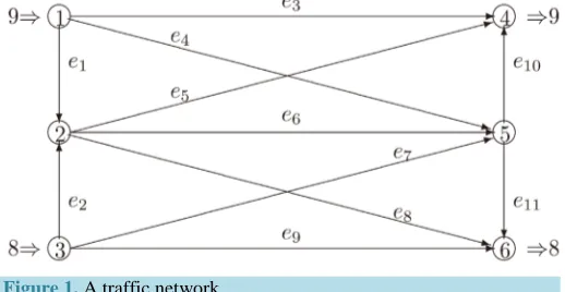
= ∅, go to Step 5; otherwise let Hi+1=HiSi+1,i= +i 1 and go to Step 2. Step 5. The equilibrium flow is fi+1 for the TEPCCA and stop.

The following example shows the calculation process of the algorithm. Example 4.1. Consider the TEPCCA (seeFigure 1), where

{

1, 2, 3, 4, 5, 6

}

V = , E=

{

e e e e e e e e e e₁, ₂, ₃, ₄, ₅, ₆, ₇, ₈, ₉, ₁₀,e₁₁

}

, C=

(

6, 7,10,8, 7, 5, 9, 7, 9,11, 7

)

,

{

1, 2

} ( ) ( )

{

1, 4 , 3, 6

}

W = ω ω = , D=

(

d_ω₁,d_ω₂

) ( )

= 9,8 , and

( )

1 1 1 2 2 2 3 3 3 4 4 4

5 5 5 6 6 6 7 7 7 8 8 8

9 9 9 10 10 10 11 11 11

2 2 2 2

2 2 2

4 17, 3 18, 30 120, 2 84,

112, 2 18, 8 62, 6 65,

18, 15, 2 10.

e e e e e e e e e e e e

e e e e e e e e e

t f f t f f t f f t f f

t f f t f f t f f

= + = + = + = +

= + = + = +

For O-D pair ω1=

( )

1, 4 : P_ω₁ contains paths l₁=

( )

e₃ , l₂ =

(

e e_{4 10}

)

, l₃=

( )

e e_{1 5} , and l₄=

(

e e e_{1 6 10}

)

, and for O-D pair ω2=

( )

3, 6 : P_ω₂ contains paths l₅ =

( )

e₉ , l₆=

(

e e_{7 11}

)

, l₇ =

(

e e_{2 8}

)

and l₈=

(

e e e_{2 6 11}

)

.

Let f =

(

f₁,f₂,f₃,f₄,f₅,f₆,f₇,f₈

)

T∈R+8, where fj denotes the flow on path lj

(

j=1, 2, 3, 4, 5, 6, 7,8

)

. Thus, we have

1 3 4, 2 7 8, 3 1, 4 2, 5 3, 6 4 8,

e e e e e e

f = f + f f = f + f f = f f = f f = f f = f + f

7 6, 8 7, 9 5, 10 2 4, 11 6 8

e e e e e

f = f f = f f = f f = f + f f = f + f .

Next, we compute the equilibrium flow with capacity constraints of arcs. 1) It is easy to verify that

(

) (

T

)

T

0

1, 2, 3, 4, 5, 6, 7, 8 9, 0, 0, 0,8, 0, 0, 0

f = f f f f f f f f = ∈A.

{

}

{ }

0 0

1 5

: l 0 ,

H = ∈l K f > = l l . Let i=0. 2) Solve the restricted problem Q0:

( )

3 3

1 1 5 5

0

1

5

1

Min d 10 120 18

3 9

. .

8

a

f

a a E

z f t x x f f f f

f s t

f

∈

= = + + +

=   = 

∑ ∫

We obtain solution f1= f0∈A. For O-D pair ω1=

( )

1, 4 , τ_ω1₁=2550, and for O-D pair ω2=

( )

3, 6 ,

1 2 82 ω

[image:4.595.184.443.584.718.2]

τ = .

(5)

3) There is no saturated arc of flow f1 in the network ℵ. For O-D pair ω1=

( )

1, 4 , it is easy to verify that the shortest path is l₄, whereas for O-D pair ω2=

( )

3, 6 , the shortest path is l₈. Note that

( )

4 8

1 1 1 1

1 2

50 2550, 46 82

l l

t f = <τω = t f = <τω = ,

thus Sω11=

{ }

l4 ,Sω12=

{ }

l8 .

4) Since S1=S_ω1₁S_ω1₂ =

{ }

l l₄,₈ ≠ ∅, let H1=H0S1 =

{

l l l l₁, , ,₄ ₅ ₈

}

and solve the restricted problem

1

Q :

( )

(

)

(

)

(

)

2

3 3

1 1 4 4 4 8 4 8

0

3 3 3 3

4 4 5 5 8 8 8 8

2

3 3 3 3

1 1 4 4 4 8 5 5 8 8

1 4

5 8

4 8

1 4 5

4

Min d 10 120 17 18

3

1 1 2

15 18 18 10

3 3 3

5 1 5

10 120 50 18 46

3 3 3

9 8 . .

5

10 0, 6 0, 9 0, 7

a f

a a E

z f t x x f f f f f f f f

f f f f f f f f

f f f f f f f f f f

f f f f s t

f f

f f f

∈

= = + + + + + + +

+ + + + + + + +

= + + + + + + + + + + =

+ = + ≤

≥ ≥ ≥ ≥ ≥ ≥ ≥

∑ ∫

8 0

f

    

 _≥



We obtain solution f2 =

(

4, 0, 0, 5,8, 0, 0, 0

)

T∈A. For O-D pair ω1=

( )

1, 4 , 2 1 600 ω

τ = , and for O-D pair

( )

2 3, 6

ω = , 2 2 82 ω

τ = .

5) After deleting saturated arc e₆ of flow _f2_{in the network}_ℵ_{. For O-D pair}ω₁₌

( )

_{1, 4} _{, it is easy to}

verify that the shortest path is l₂, whereas for O-D pair ω2=

( )

3, 6 , the shortest path is l₅. Note that

( )

2 5

2 2 2 2

1 2

124 600, 82 82

l l

t f = <τω = t f = =τω = ,

thus Sω2₁ =

{ }

l₂ ,Sω2₂ = ∅.

6) Since S2 =Sω2₁Sω2₁=

{ }

l₂ ≠ ∅, let H2 =H1S2 =

{

l l l l l1, , , ,2 4 5 8

}

and solve the restricted problem

2

Q :

( )

(

)

(

)

(

)

(

)

(

)

(

)

2

3 3

1 1 4 4 4 8 4 8

0

3 3 3 3 3

2 4 2 4 2 2 5 5 8 8 8 8

2 3

3 3

1 1 4 4 4 8 2 4

3 3 3

2 2 5 5 8 8

1 2 4

4

Min d 10 120 17 18

3

1 2 1 2

15 84 18 18 10

3 3 3 3

4 1

10 120 50

3 3

2 1 5

99 18 46

3 3 3

. .

a f

a a E

z f t x x f f f f f f f f

f f f f f f f f f f f f

f f f f f f f f

f f f f f f

f f f

s t

∈

= = + + + + + + +

+ + + + + + + + + + + +

= + + + + + + +

+ + + + + + + +

∑ ∫

5 8

2 4

4 8

1 2 4 5 8

9 8 11 5

10 0, 8 0, 6 0, 9 0, 7 0

f f f f f f

f f f f f

= 

 + =  ₊ _≤ 

 + ≤ 

≥ ≥ ≥ ≥ ≥ ≥ ≥ ≥ ≥ ≥ 

We obtain solution 3

(

)

T

1.44, 3.64, 0, 3.92, 6.92, 0, 0,1.08

f = ∈A. For O-D pair ω1=

( )

1, 4 , 3

1 182.20 ω

τ = , and for O-D pair ω2=

( )

3, 6 , 3

2 65.89

ω

τ = . 7) After deleting saturated arc e₆ of flow 3

f in the network ℵ. For O-D pair ω1=

( )

1, 4 , it is easy to ve-rify that the shortest path is l₂, whereas for O-D pair ω2=

( )

3, 6 , the shortest path is l₅. Note that

( )

2 5

3 3 3 3

1 2

182.20 182.20, 65.89 65.89

l l

t f = =τ_ω = t f = =τ_ω = , thus 3 3

1 , 2

(6)

8) Because 3 3 3

1 2

S =Sω Sω = ∅, the equilibrium flow is

(

)

T 3

1.44, 3.64, 0, 3.92, 6.92, 0, 0,1.08

f = , hence

stop. Note that

( )

(

)

(

)

(

)

( )

(

)

(

)

(

)

( )

(

)

( )

(

)

1 1

1 1 1

2 2

2 2 2

3 3

3 3 3

4 4

4 4 4

3

2 3

3 4 3 4

0 0

3

2 3

7 8 7 8

0 0

2 3 3

1 1

0 0

2 3

0 0

4 4

d 4 17 d 17 17 ,

3 3

d 3 18 d 18 18 ,

d 30 120 d 10 120 10 120 ,

2

d 2 84 d 84

3 e e e e e e e e f f

e e e

f f

e e e

f f

e e e

f f

e e e

t x x x x f f f f f f

t x x x x f f f f

t x x x x f f

= + = + = + + + = + = + = + + + = + = + = + = + = +

∫

( )

(

)

( )

(

)

(

)

(

)

( )

(

)

( )

(

)

5 5

5 5 5

6 6

6 6 6

7 7

7 7 7

8 8

3

2 2

2 3 3

3 3

0 0

2 2

4 8 4 8

0 0

2 3 3

6 6 0 0 2 3 0 0 2 84 , 3 1 1

d 112 d 112 112 ,

3 3

d 2 18 d 18 18 ,

8 8

d 8 62 d 62 62 ,

3 3

d 6 65 d 2 65

e e

f f

e e e

f f

e e e

f f

e e e

f f

e e

f f

t x x x x f f f f

t x x x x f f

= + = + = + = + = + = + = + + + = + = + = + = + = +

∫

( )

(

)

( )

(

)

(

)

(

)

( )

(

)

(

)

(

)

8 9 9

9 9 9

10 10

10 10 10

11 11

11 11 11

3

7 7

2 3 3

5 5

0 0

3

2 3

2 4 2 4

0 0

3

2 3

6 8 6 8

0 0

2 65 ,

1 1

d 18 d 18 18 ,

3 3

1 1

d 15 d 15 15 ,

3 3

2 2

d 2 10 d 10 10 .

3 3 e e e e e e e f f

e e e

f f

e e e

f f

e e e

f f

t x x x x f f f f

= + = + = + = + = + = + = + + + = + = + = + + +

∫

Thus the generalization of Beckmann’s formula Q is:

( )

(

)

(

) (

)

(

)

(

)

(

)

(

)

(

)

(

)

(

)

3 3 3

3 4 3 4 7 8 7 8 1 1

2

3 3 3

2 2 3 3 4 8 4 8 6 6

3 3

7 7 5 5 2 4 2 4 6 8 6 8

1 2 3 4

5 6 7 8

2 4

3 4

6

4

Min 17 18 10 120

3

2 1 8

84 112 18 62

3 3 3

1 1 2

2 65 18 15 10

3 3 3

9 8 11 6 . .

z f f f f f f f f f f f

f f f f f f f f f f

f f f f f f f f f f f f

f f f f

f f

s t f

= + + + + + + + + + + + + + + + + + + + + + + + + + + + + + + + + + + = + + + = + ≤ + ≤ 8 7 8 4 8

1 2 3 4

5 6 7 8

7 7 5

10 0, 8 0, 6 0, 5 0,

9 0, 7 0, 7 0, 5 0.

f

f f

f f f f

      ₊ _≤   + ≤  + ≤   ≥ ≥ ≥ ≥ ≥ ≥ ≥ ≥   ≥ ≥ ≥ ≥ ≥ ≥ ≥ ≥ 

It is easy to verify that f =

(

1.44, 3.64, 0, 3.92, 6.92, 0, 0,1.08

)

T is the solution of the generalization of Beck-mann’s formula Q

(

Minz f

( )

=1327.31

)

. Clearly, f is an equilibrium flow for the TEPCCA.

(7)

Acknowledgements

This work was supported by National Natural Science Foundation of China (Grant No. 11271389).

References

[1] Wardrop, J. (1952) Some Theoretical Aspects of Road Traffic Research. Proceedings of the Institute of Civil Engineers,

Part II, 1, 325-378. http://dx.doi.org/10.1680/ipeds.1952.11362

[2] Beckmann, M.J., McGuire, C.B. and Winsten, C.B. (1956) Studies in the Economics of Transportation. Yale Universi-ty Press, New Haven.

[3] Chen, G.Y. and Yen, N.D. (1993) On the Variational Inequality Model for Network Equilibrium [Internal Report 3. 196 (724)]. Department of Mathematics, University of Pisa.

[4] Lin, Z. (2010) The Study of Traffic Equilibrium Problems with Capacity Constraints of Arcs. Nonlinear Analysis: Real World Applications, 11, 2280-2284. http://dx.doi.org/10.1016/j.nonrwa.2009.07.002

[5] Lin, Z. (2010) On Existence of Vector Equilibrium Flows with Capacity Constraints of Arcs. Nonlinear Analysis, 72, 2076-2079. http://dx.doi.org/10.1016/j.na.2009.10.007

[6] Xu, Y.D. and Li, S.J. (2014) Vector Network Equilibrium Problems with Capacity Constraints of Arcs and Nonlinear Scalarization Methods. Applicable Analysis: An International Journal, 93, 2199-2210.

http://dx.doi.org/10.1080/00036811.2013.875160

[7] Chiou, S.W. (2010) An Efficient Algorithm for Computing Traffic Equilibria Using TRANSYT Model. Applied Ma-thematical Modelling, 34, 3390-3399. http://dx.doi.org/10.1016/j.apm.2010.02.028

[8] Xu, M., Chen, A., Qu, Y. and Gao, Z. (2011) A Semismooth Newton Method for Traffic Equilibrium Problem with a General Nonadditive Route Cost. Applied Mathematical Modelling, 35, 3048-3062.

http://dx.doi.org/10.1016/j.apm.2010.12.021