Prediction of Ground Water Level in Arid Environment Using a Non Deterministic Model

http://dx.doi.org/10.4236/jwarp.2014.67064

Prediction of Ground Water Level in Arid

Environment Using a Non-Deterministic

Model

Mohammad Mirzavand1, Seyed Javad Sadatinejad2, Hoda Ghasemieh1, Rasool Imani1,

Mehdi Soleymani Motlagh1

1_{Department of Natural Resources and Geoscience, University of Kashan, Kashan, Iran} 2_{Department of New Sciences and Technologies, University of Tehran, Tehran, Iran}

Email: [email protected]

Received 9 March 2014; revised 5 April 2014; accepted 2 May 2014

Copyright © 2014 by authors and Scientific Research Publishing Inc.

This work is licensed under the Creative Commons Attribution International License (CC BY). http://creativecommons.org/licenses/by/4.0/

Abstract

Modeling and forecasting of the groundwater water table are a major component of effective planning and management of water resources. One way to predict the groundwater level is analy-sis using a non-deterministic model. This study assessed the performance of such models in pre-dicting the groundwater level at Kashan aquifer. Data from 36 piezometer wells in Kashan aquifer for 1999 to 2010 were used. The desired statistical interval was divided into two parts and statis-tics for 1990 to 2004 were used for modeling and statisstatis-tics from 2005 to 2010 were used for vale-diction of the model. The Akaike criterion and correlation coefficients were used to determine the accuracy of the prediction models. The results indicated that the AR(2) model more accurately predicted ground water level in the plains; using this model, the groundwater water table was predicted for up to 60 mo.

Keywords

Non-Deterministic Models, Akaike Criterion, Ground Water Level, Kashan Aquifer

1. Introduction

such as the flow rate of a river. The purpose of hydrological studies is to quantitatively describe the statistical population; the process of creating this statistical population was based on a limited number of samples [2]. Random time series have been applied to solving hydrological issues by Brass and Rodriguez (1985) [3]; Berkol and Davis (1987) [4], and Lin and Lee (1994) [5]. Mathematical modeling of time series can produce hydro-logical synthetic data, predict hydrohydro-logical events, identify trends and shifts in data, complete a missing data, and generate data. The output of artificial series from river flows for drought and flood studies have been used to optimize utilization of reservoir systems and design the capacity for water supply systems [2] [6], among other uses. One basic hypothesis for modeling time series is that time series is stationary. A time series with its own statistical parameters (e.g., mean and variance) is considered stationary when its expected value is time-inde- pendent. The expected value is the average value which would be expected if the processes were repeated an in-finite number of times. More formally, the expected value is a weighted average of all possible values. Many hy- drological time series are non-stationary for reasons such as climate change, drought, and statistical parameters such as mean and standard deviation. To increase knowledge about methods of statistical determination, it could be useful to remove stationary and non-stationary time series [7]. Factors that may cause non-static time series include periodic or seasonal trends and shifts [8]. Static tests can detect the impact of each factor on a stationary time series; however, non-stationary examinations of time series can aid understanding of the physical mecha-nisms, which indicate the impotence of static tests on hydrological time series analysis (Wang et al., 2005) [9]. Stationary time series analysis methods generally fall into two categories. The first category consists of me- thods based on the analysis if there is a statistical difference in segments of a time series. In the second category, the static test is based on the statistical properties of the whole time series [10]. Numerous studies have been done in the field of hydrology based on time series, such as Javidi and Sharifi (2009), who used time series to predict the mean annual flow rate of a river. Evaluation of time series models using the Akaike information cri-terion (AIC) and residual variance has concluded that the autoregressive (2) (AR (2)) model is more appropriate for data production, thus, it was chosen as the final model [11]. Khalili et al. (2010) investigated the trends and stationary analysis of river flow in Urumia province for Shahr Chay River using KPSS and ADF methods. Their results showed that the annual flow rate series was static at a significance level of 5% [7]. Golmohammadi and Safavi (2010) used univariate hydrological time series and a fuzzy system based on adaptive neural networks to predict the flow rate of Zayandehrood, the largest river in the central plateau of Iran. The results indicated the efficiency of these systems in the forecast [12]. Nakhaei and Mirarabi (2010) used the Box-Jenkins model to predict floods using series data to determine the flow rate for Sumar in Kermanshah province of Iran. Box-Jen- kins applies the autoregressive moving average (ARMA or ARIMA) models to finding the best fit of a time se-ries to past values in order to make forecasts. They used trial-and-error criteria of residual and selected the best model among the models examined (ARMA (1, 1, 0) (2, 2, 1) (1, 2)) to predict river flow rate for the next 24 months [13]. Ahan (2000) predicted water table fluctuations using ARIMA models. According to the data, he used the quadratic difference method to remove the trend in time series [14]. Saeidian and Ebadi (2004) deter-mined the time series model for the flow rate of Talkhehrood river in northwestern Iran. They fitted time series patterns for over 53 years of flow rate data to the AIC test and determined that the best model was the AR(2)

[15]. Jalali (2002) provided decision support systems (DSS) for repositories of time series models to forecast the input of monthly flow rate for Jiroft Damin Kerman Province using a single-univariate ARIMA model to cali-brate the input flow rate [16]. Alonekyenak (2007) examined the performance of artificial neural network mod-els and the ARMA model to predict the level of water for a time period of more than 1 mo [17]. Amabyl et al. (2008) fitted time series models to simulate data obtained from the SWAT model and historical data. They found that the groundwater table data performed well in time series models [18]. The present study used the re-sults of previous research and the ability of time series techniques for time series analysis to determine the opti-mal model and used it to predict the water table of an aquifer and determine the accuracy of predictions.

2. Methods

2.1. Study Area Choice

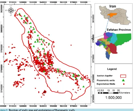
The study area (longitude: 51˚32' to 51˚03'E, latitude: 33˚27' to 34˚13'N) is located in Kashan plain, Esfahan province, Iran (Figure 1).

Figure 1. Position of study area and exploitation of Piezometric wells.

range to the south by the Natanz plains and to the east by the Salt Lake range. It has an area of approximately 7083 km2_{, of which 3040 km}2 _{consists of highlands and 4043 km}2 _{consists of submontane regions to the north} and northeast. The area under study is the Kashan aquifer located in the Kashan plain, which is 1570.23 km2 _in size (Figure 1). The annual evaporation range is 2100 to 3000 mm and the average of annual humidity is about 42 percent. Maximumtemperaturesin the summer, the warmest month (July) to 48˚C and a minimum tempera-ture of −5˚C inthewintertocome. Annual rainfall is varied in salt lake with 75 mm at the east to 300 mm in the southwest mountains. The Kashan aquifer in unconfined aquifer and because of largely discharge from this aq-uifer for agriculture, industry and drinking, The Kashan aqaq-uifer experiences an average annual loss of about 0.57 m and a critical negative budget (about −32 million m3 _{annual discharge).}

Figure 2. Time series diagram with random, seasonal and trend components.

2.2. Auto-Regressive Model

Researchers such as Slutsky (1937), Walker (1931), Yaglom (1955), and Yule (1927) first formulated the con-cept of Auto-Regressive (AR) and moving average (MA) [1]. These models are stochastic conventional models and as their name implies, imposes regression on its sentences; however regression is performed for past values of zt. This model is applicable for stationary and non-stationary time series and the basic structure is suggested

in Equation (1):

1 1 2 2

t t t p t p t

z =φz− +φ z− + + φ z− +a (1) In the above equation, φ1, φ2, φp and ... are coefficients and parameters of the AR model and at is random.

The remaining time-independent (noise) obeys a normal distribution with a mean of zero. In this model, if

0 j

j

φ ∞

=

∑

2.3. Moving Average Model

The general form of the moving average (MA) model with q rank can be expressed as Equation (2):

1 1 2 2

t t t q t q t

z =θa− +θ a− + + θ a− +a (2) where θ1, θ2, θq are the coefficients and parameters of the MA model [11].

2.4. General Structure of ARMA Model

The ARMA (p,q) model was created by combining the AR (p) model and the MA (q) model. The general struc-ture of ARMA can be expressed as Equation (3):

1 1 2 2 1 1 2 2

t t t p t p t t t q t q

nary in reality; therefore, we can model time series with the static subtraction operation and then an AR or MA model or a complex pattern can be fitted to the differencing series. The result for the non-differential series is a comprehensive model (ARMIA) [20].

2.5. Box-Jenkins Seasonal Pattern ARIMA Model

Non-seasonal time series models in the interconnected autoregressive model are moving averages and are dis-played as ARIMA (p,d,q). In this model, p represents the autoregressive model, q represents the moving average model, and d represents data differencing. For a stationary time series, d = 0 and the ARIMA model converts to ARMA. The general multiplicative seasonal pattern can be expressed as Equation (4):

( )

( )

( )

( )

p B p B Wt q B Q B at

φ Φ =θ Θ (4)

where B is the shift operator, and φp, Φp, θq, ΘQ are the polynomials of p, p, q, respectively, and at is used

instead of zt (Box-Jenkins) and is a purely random process with a mean of zero and σa2 variance. Variables of

the initial set to eliminate trends and seasonality can be expressed as Equation (5):

12

d D

t t

W = ∇ ∇ X (5) In the ARIMA model, where data differencing occurs d represents non-seasonal differencing. With non-sea- sonal differencing (D), the ARIMA model is converted to a SARIMA model. The ARIMA time series is the most complete is commonly used. A more detailed discussion about its usage can be found in Box and Jenkins (1976) [19]. Studies by Vangyr and Zoor (1997), Knotters and Vanvalsom (1997) [20], and Ahan (2000) [14]

suggest that the Box-Jenkins model for time series is an appropriate model for investigating the behavior of groundwater.

2.6. Determining the Best Model

The properties of the autocorrelation coefficients and partial autocorrelation are other criteria that determine the best model for the time series using AIC. The test is used for comparison of different ARMA (p,q) models and is calculated as Equation (6):

(

)

( )

(

)

AIC p q =N σε + p q (6)

erehw N is the amount of time series data and 2

ε

σ is the variance of error (residuals). The model with lower AIC is the more appropriate model [21] [22]. In addition to testing for AIC, the length of the forecast for the sta-tistical mean and correlation test are used. The results are shown in Table 1. After choosing the appropriate model, the predicted data are normalized and examined using the Kolmogorov-Smirnov model. The data used in this study were monthly; delays for these models were for 12 mo.

3. Results & Discussion

The results of determining a trend in the data and deterministic and random terms (Figure 2) to determine auto-correlation and partial autoauto-correlation functions before removal and data differencing (Figure 3). The results for different models are shown in Table 1. Models that fit the time series to forecast groundwater level changes are shown in Figure 4. Figure 5 valuates the correlation between the observed and predicted values by the selected models. Figure 5 shows autocorrelation and partial autocorrelation functions for predicted data by the selected models.

In this study, 5 models using 11 time series structures were examined. For each parameter, AIC and correlation coefficients for the coming months were obtained (Table 1).

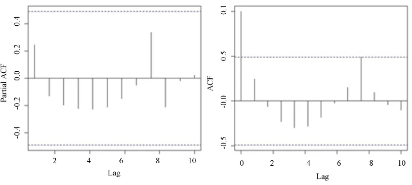
Figure 3. (a) Auto-correlation and (b) partial auto-correlation functions of the monthly groundwater level time series before removal of trends and data differencing.

Figure 4. (a) Models prediction versus observed and final model correlation (b).

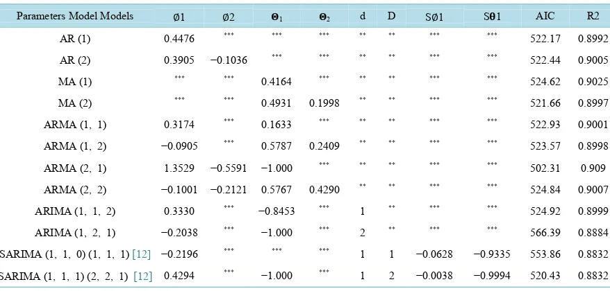
Table 1. AIC coefficient, parameters and different models used to choose the final model.

R2 AIC S𝛉𝛉1

S∅1 D d 𝚯𝚯2 𝚯𝚯1 ∅2 ∅1

Parameters Model Models

0.8992 522.17 *** *** ** ** *** *** *** 0.4476 AR (1) 0.9005 522.44 *** *** ** ** *** *** −0.1036 0.3905 AR (2) 0.9025 524.62 *** *** ** ** *** 0.4164 *** *** MA (1) 0.8997 521.66 *** *** ** ** 0.1998 0.4931 *** *** MA (2) 0.9001 522.93 *** *** ** ** *** 0.1633 *** 0.3174 ARMA (1, 1)

0.8998 523.57 *** *** ** ** 0.2409 0.5787 *** −0.0905 ARMA (1, 2)

0.909 502.31 *** *** ** ** *** −1.000 −0.5591 1.3529

ARMA (2, 1)

0.9007 524.84 *** *** ** ** 0.4290 0.5767 −0.2121 −0.1001 ARMA (2, 2)

0.8999 524.92 *** *** ** 1 *** −0.8453 *** 0.3330 ARIMA (1, 1, 2)

0.8884 566.39 *** *** ** 2 *** −1.000 *** −0.2038 ARIMA (1, 2, 1)

0.8832 553.86 −0.9335 −0.0628 1 1 *** *** *** −0.2196 SARIMA (1, 1, 0) (1, 1, 1)[12]

modeling. In this study, 5 models with 11 different structures are examined. According to Figure 3, obtained be-fore removing deterministic components of the data; it was found that the groundwater depth data has a seasonal trend and it was used to eliminate the trend and create the stationary series used various models. As seen from Figure 4(a), Figure 4(b), the autocorrelation function is exponentially reduced and also, partial autocorrelation function is not significant after a lag. According to the interpretation of these two functions can say at first sight that by using these data the AR model is an appropriate model to predict, but for a more accurate prediction, the Akaike criterion and the correlation coefficient were used to select the final model. The results of various models survey based on test and the Akaike criterion (AIC), which is one of the common methods to compare different models especially ARMA time series, also based on amount of model parameters and correlation coefficients were determined. Between mentioned models, appropriate model is firstly that an amount of the absolute value does not to exceed of 1 and the second it has lowest Akaike criteria (Table 1).

Thus, among 11 studying structure based on Akaike criterion and model parameters, the model ARMA (2,1) due to violation of model parameters of 1 were deleted between studying model. Among the remain models; SARIMA model (1, 1, 1) (1, 1, 1) [12] had the lowest Akaike criterion but to examine the results of Akaike crite-rion for this model (as mentioned in above, Akaike critecrite-rion is to test the ARMA models) correlation test was used. As shown in Table 1, based on Akaike test SARIMA (1, 1, 0) (1, 1, 1) [12] model has less Akaike statistic value but based on the results of the correlation test had less accuracy of predictions in compared other models. For this reason, another model which had less Akaike and in terms of the correlation coefficient had meaningful predictions was selected. Therefore AR (2) model was selected as the final model, to predict changes in water ta-ble levels of Kashan plain for 60 months ahead .The Kolmogorov-Smirnov test was used to examine the normal-ity of the predicated data. The significance was greater than 0.5 (sig = 1), allowed acceptance of the null hypothe-sis, meaning the normality of predicted data. Figure 5 shows that the autocorrelation function and partial auto-correlation with 10 time lags after removing the trend data were significant. From the results of studies by Karamooz and Iraqi (2005) [8], Hashemi and Jahanshahi (2005) [22], Javidi and Sharifi (2009) [11], and Nakhaei and Mirarabi (2010) [13] and the results of this study, it can be concluded that the model selected to predicted the function is important and the output is very good. AIC results for all models except the Box-Jenkins model, gave appropriate statistics. It is better use the correlation coefficient to test the models for accuracy of their predictions for the time interval. According to the non-deterministic and randomness nature of hydrological issues, time se-ries are an appropriate technique to forecast hydrological phenomena. According to the results of this research on time series models, for cases were sufficient data is not available, to generate data and predict changes in hydro-logical variables, time series models can be used. These models can be used to optimize models, for accurate pre-dictions and proper planning, and to obtain reliable management for any area.

4. Conclusion

In this study, the prediction models that were developed with standard logistic regression analysis in groundwater

level data were compared. According to the non-deterministic and random nature of the hydrological issues, time series is one of the appropriate methods to forecast hydrological phenomena.

References

[1] De Gooijer, J.G. and Hyndman, R.J. (2006) 25 Years of Time Series Forecasting. International Journal of Forecasting, 22, 443-473. http://dx.doi.org/10.1016/j.ijforecast.2006.01.001

[2] Salas, J.D. (1993) Analysis and Modeling of Hydrological Time Series. In: Maidment, D.R., Ed., Handbook of Hy-drology, McGraw-Hill, New York, 19.1-19.72.

[3] Brass, R.L. and Rodriguez-lturbe, L. (1985) Random Functions and Hydrology. Addison-Wesley Publishing Company, Reading.

[4] Brockwell, P.J. and Davis, R.A. (1987) Time Series: Theory and Methods. Springer-Verlag, New York. http://dx.doi.org/10.1007/978-1-4899-0004-3

[5] Lin, G.F. and Lee, F.C. (1994) Assessment of Aggregated Hydrologic Time Series Modeling. Journal of Hydrology, 156, 447-458.

[6] Salas, J.D., Delleur, J.W., Yevjevich, V. and Lane, W.L. (1980) Applied Modeling of Hydrologic Time Series. Water Resources Publications, Littleton.

[7] Khalili, K., Fakheri Fard, A., Din Pajooh, Y. and Ghorbani, M.A. (2010) Trend and Stationary Analyses of River Flow for Hydrological Time Series Modeling. Journal of Soil and Water Silences, 20, 61-72.

[8] Karamooz, M. and Aragi Nejad, S. H. (2005) Advanced Hydrology. 1st Edition, Amirkabir University of Technology Press, Tehran, 464.

[9] Wang, W., Van Gelder, P.H.A.J.M. and Vrijling, J.K. (2005) Trend and Stationary Analysis for Streamflow Processes of Rivers in Western Europe in 20th Century. IWA International Conference on Water Economics, Statistics and Fi-nance, Rethymno, 8-10 July 2005, 11.

[10] Chen, H.L. and Rao, A.R. (2003) Linearity Analysis on Stationarity Segments of Hydrologic Time Series. Journal of Hydrology, 277, 89-99. http://dx.doi.org/10.1016/S0022-1694(03)00086-6

[11] Javidi Sabaghian, R. and Sharifi, M.B. (2009) Using Stochastic Models to Simulate River Flow and Forecast Annual Average Flow of the River by Time Series Analysis. First International Conference on Water Resources, Semnan, 16-18 August 2009, 9.

[12] Golmohammadi, M.H. and Safavi, H.R. (2010) Pridicting of One-Variable Hydrological Time Series Using Fuzzy Systems Based on Adaptive Neural Network. The 5th National Congress on Civil Engineering, Mashhad, 4-6 May 2010, 8 p.

[13] Nakhaei, M. and Mir Arabi, A. (2010) Flood Forecasting through Sumbar River Discharge Time Series Using the Box —Jenkins Model. Journal of Engineering Geology, 4, 901-915.

[14] Ahan, H. (2000) Modeling of Groundwater Heads Based on Second Order Difference Time Series Modeling. Journal of Hydrology, 234, 82-94. http://dx.doi.org/10.1016/S0022-1694(00)00242-0

[15] Saidian, Y. and Ebadi, H. (2004) Time Series Model Determining for Flow Discharge Data (Case Study: Vaniar Hy-drometer Station in AjiChay River Basin). 2nd National Student Conference on Water and Soil Resources, Shiraz, 12-13 May 2004, 7.

[16] Jalali, K. (2002) Jiroft Dam Reservoir Inflow Forecasting Using Time Series Theory. 6th International Seminar on River Engineering, Ahvaz,8-10 February 2002, 9.

[17] Alonekyenak, A. (2007) Forecasting Surface Water Level Fluctuations of Lake Van by Artificial Neural Networks.

Water Resource Manage, 21, 399-408. http://dx.doi.org/10.1007/s11269-006-9022-6

[18] Amabyl, V., Gabriel, G. and Bernard, A.E. (2008) Fitting of Time Series Models to Forecast Stream Flow and Groundwater Using Simulated Data from SWAT. Journal of Hydrology Engineering, 13, 554-562.

http://dx.doi.org/10.1061/(ASCE)1084-0699(2008)13:7(554)

[19] Box, G.E.P. and Jenkins, G.M. (1976) Time Series Analysis: Forecasting and Control. Holden Day, San Francisco. [20] Knotters, M. and Van Walsum, P.E. (1997) Estimating Fluctuation Quantities from Time Series of Water Table Depths

Using Models with a Stochastic Component. Journal of Hydrology, 197, 25-46. http://dx.doi.org/10.1016/S0022-1694(96)03278-7

[21] Karamooz, M. and Aragi Nejad, S.H. (2010) Advanced Hydrology. 2nd Edition, Amirkabir University of Technology Press, Tehran, 464.