Munich Personal RePEc Archive
Interpretation of the Effects of Filtering
Integrated Time Series
Valle e Azevedo, João
21 September 2007
Online at
https://mpra.ub.uni-muenchen.de/6574/
Interpretation of the Effects of Filtering
Integrated Time Series
Jo˜ao Valle e Azevedo
∗Banco de Portugal & Universidade NOVA de Lisboa
September 21, 2007
Abstract
We resort to a rigorous definition of spectrum of an integrated time series in order to characterise the implications of applying linear filters to such series. We conclude that in the presence of integrated series the transfer function of the filters has exactly the same interpretation as in the covariance stationary case, contrary to what many authors sug-gest. This disagreement leads to different conclusions regarding the link of the original fluctuations with the transformed fluctuations in the time series data, embodied in various unjustified criticisms to the application of detrending filters. Despite this, and given the fre-quency domain characteristics of filtered macroeconomic integrated series, we acknowledge that the choice of a particular detrending filter is far from being a neutral task.
JEL Classification: E32; C22
Keywords: Unit roots, Band-pass filters, Pseudo-spectrum
1
Introduction
The failure of classical Fourier analysis in the presence of unit roots has led to widespread misunderstandings regarding the effects of applying linear filters to integrated time series. While some authors completely disregard spectral theory under non-stationarity, others resort to the
∗
Address: Av. Almirante Reis,71-6th floor, 1150-012 Lisboa, Portugal; E-mail: [email protected];
so-called pseudo-spectrum without providing a rigorous justification for its use. If we want to fully understand the consequences of applying transformations (linear filters) to integrated time series, we should be able to decide which view, if any, is correct. Hopefully, we will be able to address an apparently simple question. What are the consequences, in the frequency domain, of differencing a random walk? Or the consequences of applying trend-extraction filters, or more specifically band-pass filters, to integrated time series? These questions are recurrent in the context of business cycle analysis. What are we isolating when applying the Hodrick-Prescott (HP) filter (see Hodrick and Prescott, 1997), the Butterworth filters proposed by Gomez (2001) the Baxter and King filter (see Baxter and King, 1999) or the Christiano and Fitzgerald filter (see Christiano and Fitzgerald, 2003) to integrated time series? Are the properties of the resulting cycle components just artefacts? Can we give a rigorous description of its properties or a rigorous interpretation of the effects of such transformations? As we shall review, these questions have a trivial answer if the original series are covariance-stationary.
Our sole contribution is assembling some results in the literature as well as our own, and use them to show that the usual interpretation of the effects of filtering, summarised by the transfer function of the filter, carries over if the input series is integrated. This occurs essentially because, although the second moments of an integrated process are time-dependent (or infinite depending on the specification of initial conditions), the distribution of the (infinite) variance (that is, the spectrum) over frequencies is not time-dependent. This phenomenon occurs with various infinite variance processes. The standard representation theorems do not hold, since the variance is not a constant and the processes exhibit persistent time dependence, but the spectrum exhibits time invariance. Understanding this apparent paradox is the purpose of this paper. We will then be able to discuss various criticisms to the application of filters in integrated macroeconomic time series. We will see that most of them are unwarranted. Nonetheless, we will show that even though a rigorous interpretation of the effects of filtering is possible, choosing or designing a specific filter is far from being a neutral task.
2
The Spectrum
2.1
Stationary case
It is well known that a covariance-stationary time series can be decomposed into an infinite weighted sum of periodic orthogonal components. This is summarised in the spectral represen-tation theorem. Let {xt} be a covariance-stationary sequence with mean zero and define the spectrum of{xt} as:
Sx(ω) =
1 2π
∞
X
k=−∞
e−iωk
γ(k), −π ≤ω≤π (1)
where i2
= −1, ω denotes the frequency measured in radians and γ(k) is the autocovariance function of{xt}at lag k. It is well known (see, e.g., Brockwell and Davis, 1991) that there exists a right-continuous orthogonal increment process{z(ω),−π ≤ω≤π} such that:
i) E[(z(ω)−z(−π))(z(ω)−z(−π))∗
] =FX(ω) = ω
Z
−π
Sx(ω)dω, −π ≤ω ≤π
where ∗denotes the complex conjugate and:
ii) xt= π
Z
−π
eiωtdz(ω) a.e.
So, xt can be decomposed into an infinite weighted sum of orthogonal fluctuations, each with
frequencyω. Sx(ω) can be interpreted as the decomposition of the variance ofxtin terms of these
fluctuations. Sx(ω) contains the same information as the second order moments characterised
byγ(k), k= 0,±1,±2, .... Sx(ω) and γ(k) form a pair of Fourier transforms in that:
γ(k) =
π
Z
−π
eiωkdFx(ω) = π
Z
−π
eiωkSx(ω)dω, k = 0,±1,±2, ... (2)
If we apply a time-invariant linear filter h(L) =
∞
P
j=−∞
hjLj where Ljxt = xt−j and such that ∞
P
j=−∞
|hj|<∞ to the sequence{xt}we obtain a filtered sequenceyt=
∞
P
k=−∞
verify that the spectrum of {yt} is given by:
Sy(ω) =|h(e
−iω
)|2
Sx(ω) (3)
whereh(e−iω
) is denoted as the transfer function of the filter. The interpretation of a time series in the frequency domain, and the analysis of the consequences of filtering, is straightforward given the spectral representation theorem. However, the conditions for it to hold are rather restrictive, the assumption of covariance stationarity being the crucial one. How can we interpret the consequences of filtering an integrated time series? Can we extend somehow the relation in (3)?
Although it is straightforward toknow the consequences of filtering an integrated time series (i.e., to know exactly what the spectrum of the filtered series is once it becomes stationary), the link with the original integrated series is hard to make if no reasonable definition of spectrum of an integrated series is available. We will argue that a more general interpretation of the spectrum is available, that is, we argue that the spectral representation theorem is a restrictive way of interpreting a time series in the frequency domain. Obviously, if we extend the definition of spectrum in order to encompass integrated series, the spectrum of a covariance stationary series should still be consistent with the spectral representation theorem. That is, under both definitions the spectrum of a covariance stationary process coincides.
2.2
Integrated case
Spectral analysis of integrated time series is a difficult task given the failure of classical Fourier analysis in that case. There have been several approaches to the spectral analysis of non-stationary processes. Hatanaka and Suzuki (1967) build a spectral theory of non-non-stationary processes by focusing on finite subsets of the sequence {xt} that have finite second moments. The defined pseudo-spectrum is time-varying and closely related to the evolutionary spectra of Priestley (1981). Another approach, widely followed, is to define the power distribution of an integrated series as the limit of the spectrum of a stationary process when the smallest autore-gressive roots converge to 1 (e.g., Harvey, 1993; Den Haan and Sumner, 2004; Young, Pedregal and Tych, 1999). The pseudo-spectrum of a general ARIMA process is defined as (see Harvey, 1993):
Sx(ω) =
σ2
ε
2π
|φ−1
(e−iω
)|2
|θ(e−iω
)|2
|1−e−iω|2s =
σ2
ε
2π
|ψ(e−iω
)|2
where xt satisfies:
φ(L)(1−L)sx
t=θ(L)εt, ∀t
σ2
ε is the variance of the white-noise innovations εt, we assume the roots of φ(L) lie outside the
unit circle and are different from those of θ(L), ψ(L) = φ(L)−1
θ(L) and s > 0 is the order of integration of the series. This limit is a time-invariant continuous function at all frequencies except at those associated with autoregressive roots with unit modulus. At those frequencies the pseudo-spectrum is not well-defined, there is a pole, a singularity associated with the unit roots1
. The spectrum of an integrated series is thus a functional form extension of the spectrum of stationary processes. Within this approach, the analysis of the consequences of filtering can be made, but the results hold by definition, as we shall review in section 3. No rigorous justification for the use of the pseudo-spectrum is presented. It is assumed that this function represents indeed a distribution of variance. Without further results it is merely an ad-hoc extension of the spectrum of a stationary series. If the spectral representation theorem does not hold, alternative definitions and the exploration of its properties should be done.
But recently, in an important paper, Bujosa, Bujosa and Garc´ıa-Ferrer (2002) extend the classical spectral analysis by developing an extended Fourier transform to the field of fractions of polynomials. A pseudo-autocovariance generating function is defined to account for the presence of unit roots and the corresponding extended Fourier transform is defined as the pseudo-spectrum. Within this approach, which leads to exactly the same functional forms as the limit of the stationary spectrum in (4), the pseudo-spectrum collapses to the standard spectrum when no non-stationary roots are present, since the extended Fourier transform is just the classical Fourier transform in that case. This extended Fourier transform is just the ratio of the Fourier transform of ψ(L) to that of the non-invertible polynomial (1−L)s, associated with the unit roots. This
leads to (4).
This complements and extends an earlier definition of the spectrum of non-stationary processes, provided by Solo (1992). Solo (1992) has shown that certain continuous-time, stationary incre-ment processes, possess many of the frequency domain properties of stationary processes. Cru-cially, although their variance is infinite or time-varying, they have a time-invariant spectrum, defined there as the limit of the expected periodogram. This definition is motivated by the fol-lowing observation, that we adapt to the discrete-time case. If {xt} is a stationary time series with meanµand the autocovariance functionγ(.) is absolutely summable, it can be shown (see,
1
e.g., Brockwell and Davis, 1991, p.343) that:
E[IT,x(0)−T µ
2
]→2πSx(0) as T → ∞ (5)
E[IT,x(ω)]→2πSx(ω) as T → ∞, ω6= 0
where Sx(ω) is the spectrum of xt and IT,x(ω) is the periodogram for a sample of size T. That
is, when T grows the periodogram converges to the distribution of variance as revealed by the spectral representation theorem. Solo (1992) argues that the result in (5) is a less restrictive inversion relation than that implied by (1), hence justifying the limit of the expected periodogram as a more general definition of spectrum. It would be comforting if the definition of Solo (1992) lead to functional forms as in (4). Unfortunately it does not. Valle e Azevedo (2007) provides an exact limit for the expected periodogram when the (discrete-time) time series contains one unit root (s = 1), under general conditions2,3
. The limit (divided by 2π) is the following, assuming as above thatxt follows (1−L)xt =ψ(L)εt, ∀t:
S∗
x(ω) =
σ2
ε
2π
(|ψ(e−iω
)|2
+|ψ(1)|2
)
|1−e−iω
|2 , ω6= 0 (6)
which differs from (4) due to the term|ψ(1)|2
in the numerator. Using this definition of spectrum instead of that in (4) would in general lead to different conclusions regarding the effects of applying linear filters to integrated processes. But these differences would not be dramatic after a simple normalisation, given the fact that the inverse of|1−e−iω
|2
dominates the behaviour of both Sx(ω) and Sx∗(ω) at frequencies close to the pole located at zero frequency. Consider the
simplest case, when{xt} verifiesxt−xt−1 =εt,∀twhere{εt}is a white noise sequence such that
E[εt] = 0 and V ar[εt] =σ
2
ε. We have, since ψ(e
−iω
) =ψ(1) = 1 :
S∗
x(ω) =
σ2
ε
π|1−e−iω|2, ω6= 0
which shows that the pseudo-spectrum, defined as in (6), is just proportional to the inverse of the Fourier transform of the differencing operator (1−L). However, if we apply the first difference filter to{xt}the spectrum of (1−L)xt=εt is given byσ
2
ε/2π. To perfectly maintain the relation
2
Put (1−L)xt=ψ(L)εt=
∞
P
j=−∞
ψjLj. The condition
∞
P
j=−∞
|ψj||j|α<∞ for some (small)α >0 is imposed
to guarantee this result. 3
Sε(ω) =|1−e−iω|
2
Sx(ω) as in (3) we would need to define the pseudo-spectrum of xt as:
Sx(ω) =
σ2
ε
2π|1−e−iω|2, ω6= 0
which is exactly what we obtain in (4) and seems a neutral normalisation of the (non-integrable) power distribution (if it were defined by (6)) ofxt. In this case, the first difference filter maintains
the usual interpretation, summarised by the function |1−e−iω
|2
. It attenuates low frequencies and amplifies high frequencies, thus producing a ”noisier” output series. The stationary case interpretation would also still be valid for any linear filter containing at least one unit root. But in general this normalisation is only neutral (or leads to values of the distribution close to those in (4)) at frequencies close to zero, which nonetheless dominate clearly the behaviour of an integrated time series. Formally, it can be shown (see Hurvich and Ray, 1995) that for a unit root process:
E[ 1
2πIT,x(ωj)/Sx(ωj)]→2 as T → ∞, ωj = 2πj/T (7)
where Sx(ωj) is defined as in (4) and regarded as the power distribution of xt, as is typical in
the long-memory literature (see also, e.g., Velasco, 1999). It should be noted thatj is held fixed, whereas the result in (6) is valid for any fixed ω 6= 0. It is easy to reconcile the two results. Heuristically, onceT grows,ωj approaches 0 and hence|ψ(e−iωj)|
2
approaches |ψ(1)|2
. Therefore
1
2πIT,x(ωj) approaches 2Sx(ωj), with Sx(ωj) defined as in (4). In the stationary case the limit in
(7) is just 1.
In short, the rigorous definition of pseudo-spectrum due to Bujosa, Bujosa and Garc´ıa-Ferrer (2002) is not completely consistent with that of Solo (1992) for processes containing one unit root, due to the ”slight” breakdown of the result in (5) in that case. Nonetheless, the unreasonableness of disregarding any spectral characterisation of unit root processes is clear.
3
Interpreting filtered integrated time series
3.1
Consequences of filtering
time series? What would be the link with the original time series fluctuations? These questions have been puzzling for a long time due to the insufficiencies of spectral theory in the presence of unit roots. This has led to numerous misinterpretations of the role of filtering in the behaviour of integrated time series, as we shall discuss below. Detractors of the use of commonly used filters often cite the fact that the spectral representation theorem does not hold in presence of integrated series. Those in support of their use fail to fully justify the frequency domain interpre-tation given to an integrated process. Given that we have at hand such interpreinterpre-tation, embodied in a definition of spectrum that encompasses integrated processes, we can proceed to discuss the effects of filtering an integrated time series.
It is straightforward to verify that if we apply an absolutely summable linear filterh(L) to an integrated time series xt, and this series becomes stationary, the spectrum of the filtered series
yt is given by:
Sy(ω) =|h(e
−iω
)|2
Sx(ω) (8)
where Sx(ω) is the pseudo-spectrum, defined as in (4), of the integrated series xt. That is, an
extension of the relation stated in (3) holds. This relation would always hold regardless of the validity of the pseudo-spectrum as a frequency domain description of xt. This occurs because
once the unit roots in the filter polynomial h(L) cancel those in the auto-regressive polynomial of xt, φ(L)(1 − L)s, what we get is a transformed series given by yt = h∗(L)φ
−1
(L)θ(L)εt,
where h∗(L) =h(L)/(1−L)
s. The spectrum of this series is obviously |h(e−iω
)|2
Sx(ω), even for
ω= 0. But this relation, without any further justification for the use of the pseudo-spectrum, is irrelevant for the analysis of the consequences of filtering. However, we can now state that the function |h(e−iω
)|2
has exactly the same interpretation as in the covariance stationary case. It represents the way fluctuations of xt with frequency ω are amplified or mitigated by the filter.
3.2
Band-pass filters applied to integrated series
In the remainder of the paper we will focus in the analysis of band-pass filters, filters designed to isolate specific fluctuations in the original time series. We give special attention to the HP filter and to finite sample approximations of ideal band-pass filters, given the emphasis put in these filters in the literature. We define an ideal band-pass filter for the frequencies band ]ωl, ωh[⊆ [0, π]
4
, as the filter that would perfectly eliminate the fluctuations with frequencies
4
outside this band and preserve without distortion the remaining fluctuations. The transfer function of an ideal band-pass filter B(L) is thus given by B(e−iω
) = 1 for ω ∈]ωl, ωh[ and 0
otherwise. The ideal filter can be expressed as B(L) =
∞
P
j=−∞
BjLj. The filter weights are well
known and given by:
Bo =
ωh−ωl
π , Bj =
sin[ωhj]−sin[ωlj]
πj ,|j| ≥1 (9)
It can be shown thatB(L) removes up to two unit roots, which means thatB(L) can be factored asB(L) = (1−L)2
B1(L) = (1−L)B∗(L) where B∗(1) = 0. Furthermore, we can easily conclude
that by applying an ideal band-pass filter to the integrated time seriesxt(with order of integration
s= 1), no fluctuations associated with frequencies outside the band of interest ]ωl, ωh[⊆[0, π] will
be present in the filtered series. That is, for ω 6= 0 and ω ∈]0, π]/]ωl, ωh[ we have Sy(ω) = 0 by
(8) since B(e−iω
) = 0. This is true regardless of the interpretation given to the pseudo-spectrum since (8) holds by definition. Also, we can conclude thatSy(0) = 0, even if the pseudo-spectrum
is not well defined for ω = 0. This occurs because yt = B∗(L)(1−L)xt = B∗(L)zt. Now, zt is
stationary and its spectrum well defined for all ω. Since B∗(1) = 0 the result follows. Finally,
for ω∈]ωl, ωh[ and since B(e
−iω
) = 1, we can conclude by (8) that Sy(ω) =Sx(ω). In short, the
ideal band pass filter retains its usual interpretation in the presence of one unit root. Further unit roots would be needed in the filter if we wanted to isolate some range of frequencies in a time series with order of integration greater than 1 and enforceSy(0) = 0.
account for the removal of unit roots while the HP and Butterworth filters fortunately possess that property. This means, together with the interpretation given to the pseudo-spectrum, that they can in fact be seen as band-pass filters when applied to integrated series (with sufficiently small order of integration)5
.
3.3
Discussion of criticisms to the use of band-pass filters
The comprehension of the consequences of filtering a time series (either stationary or integrated) is crucial to this analysis. Many criticisms to the HP filter and to other band-pass filters forget such consequences. For instance, differences between second moments of filtered and unfiltered series cannot be taken as evidence of a weak performance of a filter as do King and Rebelo (1993), Guay and St-Amant (1997) and Canova (1998). The differences are a consequence of filtering, since the spectrum of the filtered series changes and the relation in (2) holds. The differences would arise even if an ideal band-pass filter were used. The analyst interested in the fluctuations approximately isolated by the filter should not be concerned with these consequences. As he should not be concerned if the filter does not isolate the cycle component in an unobserved-components model with a stochastic trend, as Murray (2003) shows. This type of criticism seems redundant except if there are arguments against the usefulness of looking at a portion of the spectrum in each particular application.
A more involved type of criticism concerns the alleged spurious ciclicity induced by band-pass filters when applied to persistent time series. Pedersen (2001) has fully addressed this issue in the case when the original series is persistent but still covariance-stationary. However, he does not resort to the definition of pseudo-spectrum, essential to rigorously extend the argument to integrated series. But let us review this type of criticism. Harvey and Jaeger (1993), Cogley and Nason (1995) and Guay and St-Amant (1997) criticise the HP filter for inducing business cycle periodicity in integrated or near-integrated time series, those with the “typical spectral shape” of Granger (1966). Figure 1 shows an example of this spectral shape for a covariace-stationary series. The spectrum decreases monotonically towards π, with the power clearly concentrated in the low frequencies. A peak in the spectrum of HP filtered series, which is absent in the spectrum of the original series, is taken as evidence of Slutzky-effect (or spurious ciclicity). This peak occurs because the low frequencies clearly dominate the spectrum of a persistent time series. Once we apply a band-pass filter, and thus eliminate low frequencies, a peak in the
5
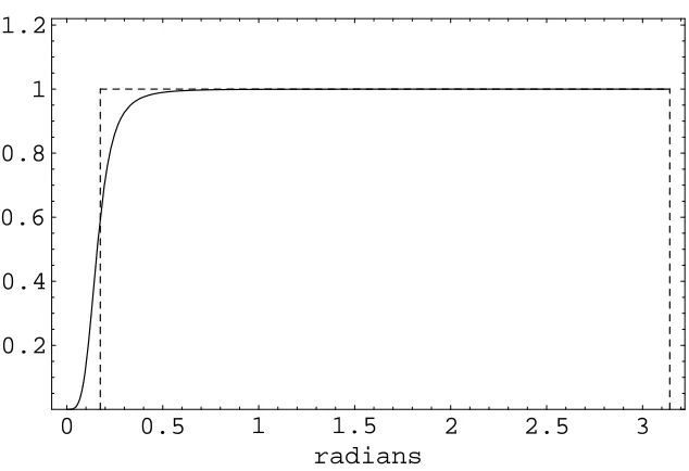
spectrum of the filtered series will be detected near the lowest frequency of the band of interest. Pedersen (2001) shows that these critics rest on an “inadequate definition of the Slutzky-effect – a definition which has the unfortunate consequence that even an ideal high-pass filter induces a Slutzky effect”. In fact, neither an ideal band-pass filter nor the commonly used band-pass filters amplify or weaken certain frequencies so as to produce a peak in the spectrum of the filtered series. They only isolate certain fluctuations that are in the data. If we define, as would be reasonable, the Slutzky-effect as a cycle in the transfer function of a filter, then the HP filter and other band-pass filters do not induce a Slutzky effect. There is clearly no cycle in the transfer function of the HP filter (see figure 2).
Crucially, the previous argument carries over to the analysis of integrated series, since we can interpret the effects of filtering integrated time series in the same way as we do for stationary processes. Many authors completely neglect this fact and analyse the consequences of filtering by first “transforming” the process into a stationary form. This completely hides or distorts relevant characteristics of the original process. E.g., Harvey and Jaeger (1993) and Cogley and Nason (1995) show that there is a peak in the power transfer function of a subcomponent of the HP filter. This subcomponent is isolated to interpret the effects of the filter inI(1) time series. Let the transfer function of the HP cyclical filter be decomposed as:
C(ω) = (1−e−iω
).C1(ω), C1(ω) =
λei2ω
(1−e−iω
)3
λei2ω(1−e−iω)4 + 1
whereλis the value of the smoothing parameter. According to this decomposition, applying the HP filter to an I(1) time series is equivalent to: First, filter the non-stationary time series with the first difference filter and then filter the remaining stationary component with the asymmetric filter determined byC1(ω) . The modulus of the transfer function of this second filter is plotted
in figure 3. It has a clear peak at business cycle frequencies that Harvey and Jaeger (1993) classify as “a classical example of the Yule-Slutzky-effect”. The definition of spectrum for an integrated process tells us that we must look to the total transfer function C(ω), not only to the subcomponent C1(ω). That is, we cannot overlook the consequences of the first-difference filter
(1−L). This introduces a complete discontinuity in the analysis of the effects of filtering once the unit root case is considered. We believe this challenges even casual observation6
.
6
We can thus state that the effects of applying a band-pass filter to an integrated series are similar to those of applying the band-pass filter to a highly persistent (but stationary) time series. The spectrum of the filtered series will have a clear peak at the lowest frequency of the band of interest, given the typical shape of the pseudo-spectrum of an integrated time series (see figure 4).
4
Choosing a specific filter is not neutral
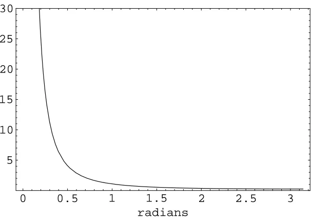
As we have seen, it is almost impossible to identify a dominant stationary component in a typical macroeconomic time series simply by looking to the pseudo-spectrum. There is not, in most cases, a clear peak in the pseudo-spectrum. It is definitely possible to have a (usually slight) peak if, e.g., the first differences of the series can be described by an AR process with complex roots. Also, if the true data generating process of the integrated series has a cycle component like the ones in Harvey and Jaeger (1993), there will be a small peak in the pseudo-spectrum at intermediate frequencies. All this means that (regular) business cycle fluctuations are hardly identified through the pseudo-spectrum. Sargent (1987) and more recently Pagan (1999), point this fact. If this was not the case we could comfortably define, in a purely statistical sense, business cycle fluctuations as those fluctuations with frequecies around the peak in the spectrum of a set of macroeconomic time series.
In view of the above, choosing to isolate a specific band of fluctuations in a macroeconomic time series (e.g., the famous [6,32] quarters band in quarterly data) or choosing a particular smoothing parameter in the case of the HP filter is essentially an arbitrary exercise, with poten-tially important consequences. Suppose for instance that a central bank uses a Taylor rule in determining interest rates, and resorts to a band-pass filter in order to estimate the output gap. The bigger the upper period in the band of interest, the more volatile will be the output gap series, since more power is being assigned to the cycle component.
Furthermore, the pseudo-spectrum is so clearly increasing as we approach the zero frequency that a cut determined by a band-pass filter will deliver a very clear peak near the lowest frequency of the band of interest, regardless of the existence of intermediate peaks. We argued before that this is not a distortion of the power distribution of fluctuations that are in the data. But it is nonetheless an important property of the filtered series.
would arise in the filtered series if the original series were a pure random walk. By applying the HP filter or another band-pass filter to a random walk process, we are again defining a trend and allowing specific frequencies to remain in the cycle component. But does it make sense to filter a random walk? Band-pass filtering is certainly “a sensible way to look at the data” (Kaiser and Maravall, 1999), just as is ideal band-pass filtering. There is no “truth” in any isolated cycle component. Prior information must be added through the specification of business cycle fluctuations. An important element of definition must therefore be assumed. As we have seen before, the peak in the spectrum of filtered series, which can be interpreted as the period of the cycle component, is mostly determined by the lowest frequency of the band of interest (or by the value of the smoothing parameter λ in the case of the HP filter). Given this important element of definition we share the view of Kaiser and Maravall (1999): “The analyst should first decide the length of the period around which he wishes to measure economic activity.” The variance of the cycle component will therefore be mostly justified by fluctuations around the critical length. A similar decision is embodied in the now standard definition of business cycle fluctuations as ”fluctuations with a specified range of periodicities” (Baxter and King, 1999)7
.
5
Conclusions
In this paper, as opposed to common practice in the literature, we have resorted to a rigorous definition of spectrum of an integrated time series in order to characterise the implications of ap-pying linear filters to such series. We show that the fact that the spectral representation theorem does not hold is not fundamental to interpret rigorously the effects of filtering integrated data. A major conclusion is that we can indeed interpret filtered integrated data in the same way as we do for stationary processes, as has been suggested by other authors. However, given the frequency domain characteristics of typical macroeconomic integrated series, we have acknowledged that the choice of a particular detrending filter is far from being a neutral task.
References
[1] Baxter, M. and King, R. (1999). Measuring business cycles: approximate band-pass filters for economic time series. Review of Economics and Statistics, 81:575–93.
7
[2] Bujosa, A., Bujosa, M. and Garc´ıa-Ferrer (2002). A Note on spectra and Pseudo-Covariance Generating Functions of ARMA processes. mimeo
[3] Brockwell, P.J. and Davis, R. (1991).Time Series: Theory and methods (2nd ed.). Springer
[4] Canova, F. (1998). Detrending and Business Cycle Facts.Journal of Monetary Economics, 41:475-512.
[5] Cogley, T. and Nason, J. (1995). Effects of the Hodrick-Prescott Filter on Trend and Dif-ference stationary time series.Journal of Economic Dynamics and Control, 19(1):253-278.
[6] Christiano, L. and Fitzgerald, T. (2003). The band-pass filter. International Economic Re-view, 44:435–65.
[7] Gomez, V. (2001). The use of Butterworth filters for trend and cycle estimation in economic time series. Journal of Business and Economic Statistics,19:365–73.
[8] Granger, C.W.J. (1966).The Typical Spectral Shape of an Economic Variable, Economet-rica, 34(1):150-161
[9] Guay, A. and St Amant, P. (1997). Do the Hodrick-Prescott and Baxter-King Filters Provide a Good Approximation of Business Cycles? . Bank of Canada, Working paper 97-53
[10] Den Haan, W.J., and Sumner, S.W. (2004). The Comovements between Real Activity and Prices in the G7. European Economic Review, 48:1333-1347
[11] Harvey, A.C. (1993).Forecasting, structural time series models and the Kalman filter. Cam-bridge University Press
[12] Harvey, A. C. and Jaeger, A. (1993). Detrending, Stylized Facts, and the Business cycle.
Journal of Applied Econometrics, 8:231-47
[13] Hatanaka, M., and M. Suzuki (1967). A Theory of the Pseudospectrum and its Application to Nonstationary Dynamic Econometric Models, in M. Shubik (ed.),Essays in Mathematical Economics in Honor of Oskar Morgenstern, Princeton, Princeton University Press.
[15] Hurvich, C.M. and Ray, B.K., (1995). Estimation of the memory parameter for nonsta-tionary or noninvertible fractionally integrated processes. Journal of Time Series Analysis, 16:17-42.
[16] Kaiser, R. and Maravall, A. (1999). Estimation of the Business cycle: A Modified Hodrick-Prescott Filter, Banco de Espa˜na -Servicio de Estudios, Working Paper 9912
[17] King, R. and Rebelo, S. (1993). Low Frequency Filtering and Real Business Cycles.Journal of Economic Dynamics & Control, 17:207-231.
[18] Murray, C. J. (2003). Cyclical Properties of Baxter-King Filtered Time Series. Review of Economics and Statistics, 85: 472-476.
[19] Pagan, A. (1999). The Getting of Macroeconomic Wisdom, mimeo, University of Melbourne.
[20] Pedersen, T. M.(2001). The Hodrick–Prescott filter, the Slutzky effect, and the distortionary effect of filters, Journal of Economic Dynamics and Control, 25:1081–1101.
[21] Priestley, M.B. (1981), Spectral Analysis of Time Series, Academic Press, London
[22] Sargent, Thomas J. (1987).Macroeconomic Theory -2nd Ed., Academic Press
[23] Solo, V.(1992). Intrinsic random functions and the paradox of 1/ f noise.SIAM Journal of Applied Mathematics, 52(1):270-291
[24] Velasco, C., (1999). Non-stationary log-periodogram regression. Journal of Econometrics, 91:325-371.
[25] Valle e Azevedo, J. (2007). Exact Limit of the Expected Periodogram in the Unit Root case, mimeo, Stanford University
0.5 1 1.5 2 2.5 3 radians 0.2
[image:17.595.136.481.137.325.2]0.4 0.6 0.8 1 1.2
Figure 1: Spectrum of a time series with the typical ”Granger” shape.
0 0.5 1 1.5 2 2.5 3
radians 0.2
0.4 0.6 0.8 1 1.2
[image:17.595.149.466.424.641.2]0 0.5 1 1.5 2 2.5 3 radians
[image:18.595.152.465.122.333.2]0.5 1 1.5 2 2.5 3 3.5 4
Figure 3: Modulus of the transfer function of the subcomponent C1(ω) of the HP cyclical filter
0 0.5 1 1.5 2 2.5 3
radians 5
10 15 20 25 30
[image:18.595.156.460.428.643.2]