The computation of distinguished hyperbolic trajectory in vector field

Journal of Chemical and Pharmaceutical Research, 2015, 7(3):2309-2319

Research Article

ISSN : 0975-7384

CODEN(USA) : JCPRC5

The computation of distinguished hyperbolic trajectory in vector field

Jia Meng

1*

and Yang Tianming

2

1_{Department of Electrical Engineering, Xin Xiang University, East Jin Sui Street, Xin Xiang City, He Nan Province,}

China

2_{Henan Institute of Science and Technology, China}

_____________________________________________________________________________________________

ABSTRACT

The computation of distinguished hyperbolic trajectory in vector field is always a hard problem. One reason is because the concept of instantaneous stagnation points trajectory (ISPT) and that of distinguished hyperbolic trajectory(DHT) are easy to be confused. Another reason is that it is hard to keep high computing speed and computing accuracy at same time. The paper first show the relationship between ISPT and DHT, then it presents to approaches to compute DHT, the advanced approach and the fast computing method.

Key words: distinguished hyperbolic trajectory; non-automatic system; measurement function, projection length _____________________________________________________________________________________________

INTRODUCTION

The development of scientific computing approaches and algorithms for the study of non-linear dynamical system behavior has long been the subject of intense research since the 1970s[1]. After several decades of development frame work of non-linear system theory has been basically achieved. Behaviors of system, such as character of attractors[2], stability[3,4] and asymptotic characteristics etc, have been made in-depth research. At present structuration theory of time-dependent aperiodic vector fields has been building, like bifurcation theory[5,6], ghosting theory[7], chaos theory[8] etc. However, the mathematical theory for both aperiodic time-dependent flows and finite time aperiodic flows is far from being a integrated system. The study of distinguished hyperbolic trajectory in time-dependent vector fields is very important in aspects of stability analysis and manifold computation[7]. So far there are mainly two methods to search for distinguished hyperbolic trajectory. K. Ide[8] proposed a method which provided an approximation to distinguished hyperbolic trajectory for entire time-interval of the data set by developing the notion of distinguished hyperbolic trajectory. And J. A. Jiménez[9] Madrid introduced a new definition of distinguished trajectories that generalized the concepts of fixed point and periodic orbit to time dependent aperiodic systems and presented numerical approach to find distinguished trajectories.

EXPERIMENT SECTION

The traditional definition of distinguished hyperbolic trajectory is as follow: Assuming x t x t( , ₀, )₀ is a trajectory of

the equation, and for each tÎ R , x t x t( , ₀, )₀ are constant in finite area. Only when x t x t( , ₀, )₀ satisfy the following conditions can it be a distinguished hyperbolic trajectory.

Condition 2, there is a neighborhood ¥ , which keeps x t x t( , ₀, )₀ in it at any time. For other initiate points in ¥ , the trajectory will leave the area either in positive or negative direction.

Condition 3, if the stable and unstable manifold of another hyperbolic trajectory form an invariant set, which contains x t x t( , ₀, )₀ , then x t x t( , ₀, )₀ must be non-hyperbolic.

For the given Measurement function, assuming the component of x t x t( , ₀, )₀ is to be

1 2

0 0

( , , ) ( ( ), ( ), , n( ))

x t x t = x t x t L x t (1)

For x_i = x t( )_i ，and n i

x Î R ，the corresponding map is : n

M R _® R+_:

2

1 ( )

( ) i

i j n t i i t j dx t

M x dt

dt t t + -= é ù ê ú = ê ú ë û

å

ò

(2)

The trajectory ( )gt is one flow of the manifold. The pointt - DT at the point on g( )t at time _{t . If the is an} *

open set ¥ which makes each x Î ¥ meet the following[18]：

* *

*

, ,

( ( )) min( ( ) )

t t

M t M x

t t

g = x Î ¥ (3)

Then the measurement function can be improved.

Distinguished trajectory can be roughly interpreted as stable manifold and unstable manifolds of intersection curve. The basic idea of Eq. (1) and Eq. (2) is that special points can be selected by comparing the arc-length of the flow in a small are. For Eq. (2), the physical meaning is in the phase space trajectory length measurement function. No matter in autonomous systems or nonautonomous systems, the timeline has been as implicit dimension. Unlike autonomous systems and nonautonomous systems is a stationary process, the influence of the timeline on system performance is more outstanding, can even nonautonomous system timeline as a separate dimension variation for autonomous systems and nonautonomous system were studied. For nonautonomous system, therefore, extended phase space than the phase space can reflect the characteristics of the details of the flow.

As Fig.1 shown, in the extended phase space of one dimension nonautonomous system , '

A A ， '

B B ， '

CC is the

projection of flowF₁， 2

F ， 3

F in the phase space. Obviously, as the value ofτ changing, _{A A ,}' _{B B and} '

'

CC can not reflect the true value of the length of F₁， 2

F ， 3

F . The physic meaning of Eq,(3) shows the

measurement function of trajectory length in extended phase space. Eq.(1) and Eq.(3) will do little effect to physical meaning of the dynamic system

2

1 ( )

( ) i 1

i j n t i i t j dx t

L x dt

dt t t + -= é ù ê ú = + ê ú ë û

å

t

x

1

F

2

F F3 A ' A B ' B C ' C t t

Fig.1 Extended phase space and phase space

To decide the initiate value, some selected area should be evaluated first. Reference[8]shown the relationship between he hyperbolic trajectory and the instantaneous stagnation points trajectory. This relationship just offers some reference to select the initiated time area to improve the approach in reference [9].

Assuming he nonlinear components_gNL( , )_{x t}r _{of the vector field is definite, and} 0 [ , ]_l

tÎ t t . We extend the vector

field in term. Then _gNL( , )_{x t}r _{can be formed into power series} ：

0

( , ) sin( ) cos( )

N NL

k k

k

g x t b k tw c k tw

=

=

_å

+

r

(5)

and

0

1

( ) sin( ) 2

l

t

k

t

b g t k t dtw p

=

_ò

0

1

( ) cos( ) 2

l

t

k

t

c g t k t dtw p

=

_ò

（6）

Example1, Assuming the vector field is as:

1 cos( )

dy

d y b k t

dt = + w (7)

The solving is :

1

1 1

0 0

2 1

2 2 2 2

1 1 1

( ) cos( ) | sin( ) |

d t

d t d t

t t

d e b bk

y t k e k e

d k d d

t w t

wt wt w - -é ù ê ú = ´ ´ + ê ú

+ _ë- _û (8)

The distinguished trajectory is :

2 1

2 2 2 2

1 1 1

( ) cos( ) sin( )

DHT

d b bk

y t k t k t

d k d d

w w w w é ù ê ú = ´ + ê ú

+ _ë- _û (9)

1

( ) cos( )

ISP

b

y t k t

d w

= - (10)

1

2 2 2

1 ( ) cos d sign b

d k q

w

=

+ (11)

1 0

( ) 0 0

1 0

b

sign b b

b

ìï <

ïï ïï

= í =

ïï

ï - >

ïïî

(12)

Then the distinguished hyperbolic trajectory can be gotten as:

( ) cos( )

DHT

y t = b k tw - q (13)

Assuming the initiate points ：

1 2

d = - ，b = 10，k = 18，w = 0.1，the simulation result is shown in

Fig.2.From Eq.(10), Eq.(12)and the simulation results we can see that ,for each harmonic of Fourier series，the difference between the distinguished hyperbolic trajectory and the instantaneous stagnation points trajectory are the magnitude and the phase delay.

When the nonlinear components_gNL( , )_{x t}r _{of the vector field is finite and it meets} 0 [ , ]_l

t Î t t , then _gNL( , )_{x t}r _{can be}

formed into power series：

0 ( , )

N

NL k

k k

g x t c t

= =

_å

r

(14)

0 1 2 3 4 5 6 7 8 9 10

-10 -8 -6 -4 -2 0 2 4 6 8 10

t

y

ISP DHT

Fig.2 the DHT and ISP of Eq.(7)

An improved method which is more sensitive to difference of measures between trajectories is proposed to compute the distinguished hyperbolic trajectory[10]. The computing process is as follows:

Step 1: According to instantaneous stagnation trajectory choose initial region. Set the initial accuracyd and the ₀

initial integral lengtht , build grid, and set initial point₀ P at time₀ t . ₀

Step 2: Change the calculation accuracy, if d_{i j,} > d, make d_j+1= d_j/ 2. If d_{i j,} < d jump into step7. Otherwise,

go to next step.

Step3: Assume P as the center and d_j+1 as accuracy of the grid to calculate the point Q . If Q ¹ P set

Step4: Consider P as the center and t₁， 2

t as integral length to calculate W1， 2

W separately, in that

1 0

t = t + D T，

2 0 2

t = t + ´ D T . If P ¹ W₁ go to next step. If P =W₁ and P ¹ W₂ jump into step 6. If

1 2

P =W =W return step 2.

Step5: Set t₀ = t₁, return step 3.

Step6: Set t₀ = t₂, return step 3.

Step7: Record the result x0 = P of time t . 0

δ

Fig. 3. Grid used in optimized algorithm

Parameter discussion:

In this paper, the approach involved many parameters. The collection of the accuracy parameter q is very important. We do some assumptions before discussion value of the accuracy parameter q .

Assumption 1 Tiny changes of the impact of computing time can be ignored.

Assumption 2 At any time t , in _i d_{i j,+1} = q d_{j i j,} ,for j∈ Ν+,q_j = q, and q is constant.

Assumption 3 Convergence point fall in the grid is equal to the probability of any position.

, i j

x is the convergence stagnation point with the accuracy of d . _{i j,} x_{i j,+1} is the convergence stagnation point with

the accuracy of d_{i j,+1}. L_{i j,} is the distance between x_{i j,} and x_{i j,+1}. d_{i j,} = qd_{i j,-1}. Then under the accuracy of

, 1 i j

d ₊ , the mesh reconstruction times from x_{i j,} to x_{i j,+1} is as follow:

, , , 1

, 1 , 1

,

, , , 1

, 1 , 1

( )

2

( )

2

i j i j i j

i j i j

i j

i j i j i j

i j i j

L L res n L L res d d d d d d + + + + + +

ì ê ú

ïï ê ú

ï <

ï ê ú

ï ê_ë ú_û ïï = í

ï é ù

ï ê ú

ï _>

ï ê ú

ïï ê_ê ú_ú ïî

(15)

And

, 1 , 1 ,

, ,

,

, 1 , 1 ,

, , , ( ) ( ) 2 ( ) ( ) 2

i j i j i j

i j i j

i j

i j i j i j

i j

i j i j

L L res res L L L res res d d d d d d d - -- -ìï ï _< ïï ïï = í

ïï _{- >}

ïï ïïî

, 1 , 1 , 1

, , ,

( i j ) i j i j

i j i j i j

L L L

res

d d d

- - ê_ê - ú_ú

= _{- ê ú}

ê ú

ë û

(17)

To minimize the computing time, and reducing the mesh reconstruction time as possible as it can.

, 1 min N i j j n =

å

dN+1< d， N

d > d (18)

d is the accuracy that satisfy our computing.

The analyze above are done for the converge points already known. For most time we don’t know the right position of the converge points, but we can get it from d computing and estimate j_{i j,} Î N . Now we do analyzing from + probability.

Because of d_{i j,+1}, the position of can only in the mesh decide by the center x_{i j,+1} and length , 1 2 i j

d ₊

. We choose

, 1 i j

L ₊ to be the expectation value of the distance.

2 1

, 1 1

1 1

( )

n

k k n

i j j

k

L ₊ x x ₊ dx dx

= W

=

-E

òò

å

L (19)

And W stands for the mesh area with the centerxi j,+1 and length , 1

2 i j

d ₊

, by assumption 3 and Eq.(17), we can

get:

, , 1

, 1

, , 1

, 1 1 ( ) 4 2 3 ( ) 4 2

i j i j

i j

i j i j

i j L res p L res d d d d + + + + æ ç _< çç çç = ç çç ç > ççè (20)

Take advantage of Eq. (18)and Eq. (19) to simplify Eq.(20).

In biaxial field, it is：

0

/

1 1 1 3

min log

2 4 2 4

d d q

q q

éê ú é ù ù_{é ù}

êê ú´ + ê ú´ ú_{êê úú} êê úë û ê úê ú ú

ë û (21)

In triaxial field, it is：

0

/

3 1 3 3

min log

8 4 8 4

d d q

q q

éê ú é ù ù_{é ù}

êê ú´ + ê ú´ ú_{êê úú} êêë úû êê úú ú

ë û

(22)

0

d is the initiate value we set before.

RESULTS AND DISCUSSION

3 dx y dt dy x x dt ìï ï = ïïï í

ïï ₌

-ïïïî

(23)

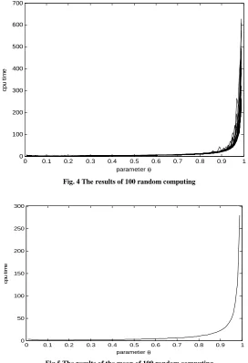
Analyzing the parameter q of differential equations (). Set the initiate accuracy d =₀ 0.2 , the computed

accuracy _{d= 10}-6_{, the initiate length of integral is 2 and the step of integral is 1. Choose 100 initiate points} randomly to do computation for parameter q in range[0.01, 0.99 . The results are seen in Fig.4. The mean of the ]

computing results can be gotten, seen from Fig.5. Fig.6 and Fig.7 show the parameter trend in biaxial and triaxial field. From Fig.5 and Fig.6, we can see the results of analyzing are Consistent with the the results of computing. This shows that for the computing of q , the advanced algorithm are consistent to different systems. Generally , we choose 0.1~0.3 for q .

0 0.1 0.2 0.3 0.4 0.5 0.6 0.7 0.8 0.9 1 0

100 200 300 400 500 600 700

parameter θ

c

p

u

t

im

e

Fig. 4 The results of 100 random computing

0 0.1 0.2 0.3 0.4 0.5 0.6 0.7 0.8 0.9 1

0 50 100 150 200 250 300

parameter θ

c

p

u

t

im

[image:7.595.156.428.204.602.2]

e

0 0.1 0.2 0.3 0.4 0.5 0.6 0.7 0.8 0.9 1 0

100 200 300 400 500 600 700 800 900 1000

parameter θ

c

o

s

t

Fig.6 The relationship between system parameter and value in biaxial field

0 0.1 0.2 0.3 0.4 0.5 0.6 0.7 0.8 0.9 1 0

100 200 300 400 500 600 700 800 900 1000

parameter θ

c

o

s

t

Fig.7 The relationship between system parameter and value in biaxial field

The fast computing method saves lots of the time while keeping the computing accuracy, which offer platform to combine the manifold analyze theory to projects[11].

If there is a hyperbolic trajectory in velocity field, and it can be defined as:

( , )

n

,

d x

v x t

x

R

t

R

d t

=

∈

∈

（24）

Assuming the trajectory passes through

x

*

at time

t

*

, then the trajectory can be presented as F (

x

*

，

t

*

，

t

). J.A .Jiménez-Madrid’s computing equation is:

*

2 *.

*

1

( )

( *)

[

]

n t

i t

t

i

d x t

M x

d t

d t

τ

τ _τ

+ −

=

=

∫

∑

（25）

the point

x

*

is more closed to DHT. The points of DHT can be approximated by using the minimal value of M when the

x

*

is closed to DHT.

For every dot on DHT, the computing steps are:

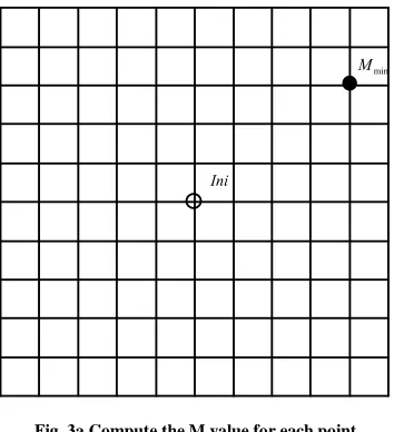
1. Drawing the 100

×

100 grids with (

x

*

，

t

*

，

t

*

) as the center and 10

δ

as the length for each grid (see Fig.3a). Then choosing proper

τ

for Eq. (24) to compute the M value for each point.

min M

[image:9.595.210.387.202.396.2]

Ini

Fig. 3a Compute the M value for each point

2. Finding the point

M

_minwhich has the minimal M value, and making it to be the center,

δ

to be the length to

draw a new 3

×

3 grids (see Fig.3b). Proper

τ

will also be chosen for Eq. (25) to compute the M value for each

point. If

M

_min still has the minimal M value, step 3 can go on, otherwise choosing

M

_new which has the minimal M value to be the center do step 2 again (see Fig. 3c ).

[image:9.595.186.409.473.585.2]

new

M

Fig. 3b Grid subdivision Fig. 3c Reset the center

3. Compute the M value for each point in grids at last we get 10

τ

instead of

τ

in step 2 for Eq. (25). If

min

M

still has the minimal M value, the appropriate point is obtained. Otherwise we choose

M

_new which has the minimal M value to be the center to do step 3 again (see Fig. 3c ).

J.A .Jiménez-Madrid spent lots of time to compute each point of DHT through the above steps. We made some improvements As follows:

* ₂ *. _*

1

( )

( *)

[

]

1

n t

i

t _t

i

dx t

M x

dt

dt

τ

τ _τ

+

− ₌

=

_∫

∑

+

（26）

Though only a little change is done, it has significant physical meanings. The new added ‘1’ equals to

dt

dt

, which means that another dimension is added to Eq. (25) to compute the real arc-length in original space. In fact, we needn’t to get the real value of the arc-length. What we need is a good measure to judge the solvers of DHT. Eq. (26) extends the space. Though it can’t get the real value, it better reflects the extend trend of the points on trajectories, as shown in Fig.4

'

L

[image:10.595.74.488.245.442.2]

L

Fig .4 Space extending

1 2

X

=

{ ( ),

x t x t

( ),... ( )}

x t

n (27)

1 2 1

X' { ( ),

=

x t x t

( ),... ( ),

x t x

n n+

=

t

}

(28)

Eq. (27) is the original space trajectory and Eq. (28) is in extended space. See Fig.4,

L

is the real value of the arc-length, but

L

'

better reflect trend of the trajectory.

In this way, the computing accuracy will be increased. Besides, for computing the point on DHT, we needn’t follow the 3 steps above. The computing accuracy depends on

δ

and

τ

. The smaller

δ

is and bigger

τ

(It has boundary. If it is too big, it will have the same effect as the small one) is, the more accuracy we will get. So we can do further subdivision to

δ

, and increase

τ

as needed to improve the computing accuracy.

CONCLUSION

The paper show two method for distinguished hyperbolic trajectory computing, the advanced method and the fast computing method. The advanced method, which based on the rapid growth of high-power function, the developed measure function. It is gained by adjusting the parameters of the existing measure function, is more sensitive to difference between measures of trajectories. Through halving the grid in each loop, the optimization algorithm could reduce convergence time, especially in low accuracy region of initial estimation. Besides, we give a discussion and confirmation that the approximate point on the local stable manifold near to special trajectory of time-dependent vector fields converges to unstable manifold in time. The fast computing method saves lots of the time while keeping the computing accuracy, which offer platform to combine the manifold analyze theory to projects. But when compute the first point, we should make sure the computing accuracy is no less than

10

−6.

REFERENCES

[3]QD Li ; XS Yang. Chin. J. Comput. Phys. 2005; 22(6): 549-554.

[4] HY Sun; YY Fan; J Zhang; HM Li; M Jia, in proccesing of International Conference on Information Science

and Technology, edited by J B He, Q H Liu, H Y Feng, N Zhang, IEEE Computational Intelligence Society,

NanJing, China (2011), p. 267.

[5] JJ Yu ; XJ Liu; WQ Han; HB Xu, Chin. J. Comput. Phys. 2004; 24(1): 116-120. [6] JA Langa ; JC Robinson; A Suarez, J. Diff. Eqs. 2006; 221: 1-35.

[7] M Branicki ; S Wiggins, Physica D 2009; 238:1625-1657.

[8] K Ide ; D Small ; S Wiggins. Nonlinear Proc. Geoph. 2002; 9: 237-263. [9] JA Jiménez ; AM Mancho, CHAOS. 2009; 19: 013111-1.

[10] WX Li; QH Ji, Computation and analysis of distinguished hyperbolic trajectories in time-dependent vector

fields,2012 International Conference on Information, Computing and Telecommunications ,2012