Characterisation of the directionality of
reflections in small room acoustics
Romero, J, Fazenda, BM and Atmoko, H
Title
Characterisation of the directionality of reflections in small room acoustics
Authors
Romero, J, Fazenda, BM and Atmoko, H
Type
Conference or Workshop Item
URL
This version is available at: http://usir.salford.ac.uk/9435/
Published Date
2009
USIR is a digital collection of the research output of the University of Salford. Where copyright
permits, full text material held in the repository is made freely available online and can be read,
downloaded and copied for noncommercial private study or research purposes. Please check the
manuscript for any further copyright restrictions.
CHARACTERISATION OF THE DIRECTIONALITY OF REFLECTIONS
IN SMALL ROOM ACOUSTICS
J. Romero1, B. Fazenda1
1
University of Huddersfield, Queensgate, Huddersfield, HD1 3DH, U.K.
ABSTRACT
This paper investigates the extraction and analysis of temporal and spatial distribution of early sound decay. A method based on B-format signals is adapted for small rooms. It can map the spatial and temporal distribution of sound energy and its diffuseness. Once the data is collected is possible to extract the information in both time and frequency domains and use this to infer issues of perception based on psychoacoustic models. The ultimate objective is to find useful descriptors for characterizing the acoustic quality in critical listening rooms.
Keywords Directionality reflections, Small room acoustics, Critical Listening rooms.
1 SPATIAL MEASUREMENT TECHNIQUES FOR SMALL ROOMS
According to theory, there are three basic types of measurements: a) Separate microphone arrays, using discrete microphone arrays where the phase relationship of signals is not preserved correctly b) Coincident microphone arrays which minimize the distance between the capsules in order to converge to a point in the space. An example of this is the Soundfield microphone which was used for the measurements. c) Intensity probe configurations (p-p probes) use a pair of measurement grade pressure calibrated capsules placed at fixed distances. The signals are processed to obtain the acoustic intensity vector along the axis where the probe is aligned.
Further advances had been reported by de Bree (2001) with a new approach based in a particle velocity (
u
) known as the Microflown probe. This solution drastically minimizes the distance between the transducers and is therefore currently the best coincident array, showing the most reliable polar pattern across frequency and the less intrusive probe up to date.The work of Merimaa et. al. (2001) and Peltonen et. al. (2001) settled the standards of extraction of directional impulse responses and diffuseness analysis with the use of perceptual issues applied to the frequency content on the signals. Later Pulkki (2007) and Ahonen et. al. (2008) expanded its uses to teleconferencing. Enroth (2007) applied these techniques for auralization of simulated acoustic impulse responses to be reproduced accurately in multiple channels. Essert (1996) developed a method based on the Soundfield microphone to measure the Lateral Energy Fraction (LEF), the Instantaneous Lateral Fraction and the Directional Fraction to describe the evolution of the sound field. The recent work of Ohta et. al. (2008) analysed reflections using a time windowing approach extracting B-Format signals from a custom microphone made of six cardioids capsules.
Fazenda (2008) used B-Format signals to extract directional distribution of reflections across time. However poor localization was found when the instantaneous acoustic intensity vector was calculated in the time domain. Therefore the motivation of using a Short Fourier Transform (STFT)approach was implemented in the present work. It should also be noted that Faller (2009) and Farina (2007) report a limitation of the Soundfield microphone for accurate estimation of reflections due to the lack of accurate first order polar patterns across the entire audible range. Above 12 kHz phase errors are present and the polar directivity of the figure of eight and the omnidirectional patterns is distorted.
3 DESCRIPTION
OF THE MEASUREMENT SYSTEM
The Soundfield SPS 422B microphone is used to extract 3-D impulse responses
2). By applying a matrix algorithm within either a hardware unit, or software implementation, it is possible to obtain the B-Format signal, which produces three orthogonal virtual figures of eight microphone polar responses centred at the origin with an additional fourth omnidirectional polar response signal which is a arbitrarily scaled down to -3 dB. For further analysis in Matlab, this is upscaled by multiplying it by root of two:
Wcorrected = 2
(
Wmeasured)
(1)This type of measurements requires a calibrated Sounfield microphone and a reliable sample and phase accurate soundcard connected to a silent portable computer. Measurement software performs the extraction of the impulse response of the four B-Format signals. (refer to figure 2). Matlab is used for further analysis discussed in Section 4. The excitation source was the existing studio monitors found in the rooms.
The impulse response of the room represents the interaction of the speaker and the room at this particular position. To obtain this a deconvolution process is performed with the aid of the
measurement software WinMLS
measurement is generated in binary or ACII file formats. The excitation signal chosen was linear swept sine. The sweep length was selected according to the measured RT, to improve accuracy. The four impulse responses were obtained by performing simultaneous RT measurements by selecting the ‘4 channel mode’, with the soundcard operating at 24 bits 96 kHz. The final step is to export data to
Matlab for further analysis using Loadimp.m, a script provided by WinMLS.
4 DATA ANALYSIS
According to Ahonen et al. (2008), the direction of arrival of the sound is opposite to the direction of the particle velocity vector
u
=u(x
,y
,z
):
2 2
XY
u
=
u
=
X
+
Y
(2)1
180º
tan
rad
Y
X
θ
π
−
−
=
−
(3)The degree of diffuseness of a sound field is a scalar value which measure the ratio between arriving directions of active intensity and energy density at a given time window. Pulkki (2007) explains that diffuseness varies between values of 0, when the direction of the incoming reflections directions is clearly determined i.e. an isolated reflection and 1, when the direction of the incoming reflections are random (implying a diffuse field). In figure 3 darker grey spot values correspond to higher values and the white values to low values of diffuseness.
Further development from Pulkki (2007) and Ahonen (2008), led to an instantaneous function of for diffusiness (ψ
) in terms of Short Term Fourier Transform windows (STFT) in a room by applying the following expression:
(
,)
1(
(
,)
)
,I n n
c E n
ω
ψ
ω
ω
= − (4)(
)
{
(
) (
)
}
0 0
1
, Re , ,
2
X
I n W n X n
c
ω
ω
ω
ρ
∗ = (5)(
)
{
(
) (
)
}
0 0 1, Re , ,
2 Y
I n W n Y n
c
ω
ω
ω
ρ
∗
=
(6)
Where ρ0 is the air density and c0 is the speed of the sound. Then matlab norm operation is applied to the Intensiy vector F n
(
,ω)
to the Expected value of intensity F n(
,ω)
= I n(
,ω)
, which in practice is calculated with the recursive integration of the STFT of the active intensity vector
I n,
( )
ω :(
)
2(
) (
) ( )
1
1
,
b
m a
I nω W n m u n m w m
=
=
∑
+ +
(7)
where W n
(
+m)
is the omnidirectional signal taken from the B-Format signal.
u n
(
+
m
)
is the particle velocity vector aligned to a particular axis and w1( )
m is a Hanning window performing a timewindowing defined between a1 and b1. The instantaneous energy density E(n,ω) is calculated by the following expression:
(
)
(
)
(
)
(
)
2 2
2 , ,
1
, ,
2 2
X n Y n
E nω W nω ω ω
+ = + (8)
In order to obtain the directions of the reflections, an STFT analysis is made to the intensity vector in the horizontal plane. The time window duration is chosen according to the sampling frequency and the ‘mean free path’ of the room. Octave band, 1/3 octave band, or Equivalent Rectangular Band (ERB) filtering can be used to smooth the time windows. The best perceptual approximation is the ERB because it resembles the human hearing resolution, whereas 1/3 octave band approximates the critical band with less accuracy and octave band may be useful for engineering analysis. The formula used to calculate the bandwidth of the rectangular filters ( ERBN ) is taken from Moore (2004):
(
3)
24.7 4.37 10 1
N
ERB = × − f+ (9)
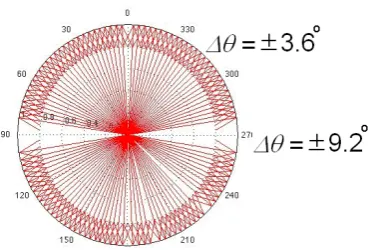
Where ERBN and frequency ( f )are in Hz. According to Venegas et. al. (2006), the Interaural Spectral Density per band between the left and the right signal is a special form of the IACC and it can obtained after filtering the signal with a bank filter that resembles the function of basilar membrane. The time domain is divided in smaller angular regions. According to Blauert’s (1997) localization blur (see figure 4). By applying small time windows to the data it is possible to analyse the early part of the decay but not the late part. This is due to the fact that reflections become too dense and they are perceived as reverberation rather than isolated discrete reflections. Nevertheless, a statistical approach is still possible in the late decay zone using selective wider time windows to cover the entire reverberant tail.
According to Buchholz et al. (2001), the perception of several room reflections are masked by the direct signal and in some cases by other loud reflections. This can be done by applying a threshold to discard the masked energy according to a psychoacoustic model. This model takes in account two variables, angle and time of arrival.
5 EXPERIMENTAL RESULTS MEASURED IN A CONTROL ROOM.
Only the horizontal plane is investigated at this time. The measurements were made in Blue Room 2 control Room, whose dimensions are 4.16 X 2.75 X 2.87 m and its volume is 32.1 m3. Measurements were performed at two different source positions. The first was at the front of the microphone and the second at 120º from the origin, referenced at front with an approximated angle of 0º (which later was measured and was 2º, see figures 1 and 3). As previously mentioned, the sampling frequency resolution was set to 96 kHz which gives a temporal resolution of 0.01 ms. For reasons of space, only one measurement is presented here.
This room has a fairly short reverberation time RT = 0.17 s @ 1 kHz, and a Mean Free Path l= 2.2 m giving a minimum time window of ∆
t
= 6 ms. However, smaller time windows of 0.1 and 1 ms were tested in this analysis and seem more appropriate to determine any isolated early reflection. For the STFT a window length of 512 points and 50% overlap was used in order to produce a smooth spectrogram (See figure 3). The time scale begins at around 139 ms, the useful region is adapted to observe the direct sound and its decay. Looking at figure 3 in the upper graph it can be seen that the variation of direction of the early reflections is not traceable after the time labelled around 150 ms. This corresponds to the 10-15 ms limit where the reflections leave the discrete zone and increase its density across time. It is interesting to see that the more diffuse the reflection, the less coherent the direction estimate is across the audible frequency range. In figure 3 it can be seen that the diffuseness values which appear as grey spots tend to vary randomly after the early reflections therefore this is not useful descriptor of the stage of decay, unless it is combined with the amplitude level of the reflections calculated with the Matlab’squiver graph function which shows the mean
direction of the reflections calculated after smoothing with the ERB bank filter. From this analysis it is clear that new measures for taking in account the mixing time and the beginning of the reverberant tail are needed in order to perform an automatic analysis of each room measured. Possibly the use of higher order statistics and modern time series theory may be adapted to cover this needs.6 CONCLUSIONS.
The estimation of direction of arrival of early reflections using the STFT approach in time-frequency domain appears to be a good technique with high accuracy and repeatability in comparison with the time domain analysis. The inclusion of Equivalent Rectangular Band bank filter and localization blur perception limits in the model helps bridge the gap between the objective measures and the subjective measures. This paper reports advances of the research up to date and possible research directions.
The physical limitation of the system is the resolution of the Soundfield microphone, especially in the forwards and backward directions where the human localisation blur angle is more accurate. The future use of the Microflown probe may improve the measurement results, and better prepare the impulse response to create accurate auralizations.
REFERENCES
AHONEN J., PULKKI V., KUECH F, KALLINGER M., SCHULTZ-AMLING R., (2008), Directional analysis of sound field with linear microphone array and applications in sound reproduction. Presented at the AES 124th Convention, Amsterdam, The Netherlands, May 17-20.
BLAUERT J., (1997), “Spatial Hearing, The Psychophysics of Human Sound Localization”, Revised Edition, MIT Press, U.S.A.
BUCHHOLZ J. M., MOURJOPOULOS J., BLAUERT J. (2001), Room Masking: Understanding and Modelling the Masking of Room Reflections. Presented at the AES 110th Conference, Amsterdam, the Netherlands, May 12-15.
DE BREE H. E., (2001), An overview of Microflown Technologies. Available at:
ENROTH S., (2007), “Spatial Impulse Response Rendering of digital waveguide mesh room acoustic simulations”. University of York, MSc Thesis.
ESSERT R., (1996), Measurement of Spatial Impulse Responses with a Soundfield Microphone. Third joint meeting of the Acoustical Society of America and the Acoustical Society of Japan Honolulu,
Hawaii, December 4-6. Available at:
August 29th 2009].
FALLER C., KOLUNDZIJA M. (2009), Design and Limitations of Non-Coincidence Correction Filters for Soundfield Microphones, AES 126th Convention, Munich, Germany, May 7–10.
FARINA A., (2007), Advancements in impulse response measurements by sine sweeps.Presented at the AES 122nd Convention, Vienna, Austria, May 5–8.
MADSEN E. R., (1970), Extraction of Ambiance Information from Ordinary Recordings. Journal of the Audio Engineering Society,Vol. 18 (5) pp. 490-496.
MERIMAA J., LOKKI T., PELTONEN T., KARJALAINEN M. (2001), Measurement, Analysis, and Visualization of Directional Room Responses. Presented at the AES 111th Convention, N.Y., U.S.A. September 21-24.
PELTONEN T., LOKKI T., GOUTARBÈS B., MERIMAA J., KARJALAINEN M., (2001), A System for Multichannel and Binaural Room Response Measurements. Presented at the AES 110th Convention, Amsterdam, The Netherlands,May 12–15.
FALLER C., KOLUNDZIJA M., (2009), Design and Limitations of Non-Coincidence Correction Filters for Soundfield Microphones. AES 126th Convention, Munich, Germany, May 7–10.
FAZENDA B., ROMERO J., (2008), 3-Dimensional Room Impulse response measurements in critical listening spaces,Proceedings of the Institute of Acoustics, Vol. 30 (6) pp. 323-239.
MOORE B.C.,(2004) “An Introduction to the Psychology of Hearing”, Fifth Edition, Elsevier, U.K. OHTA T, YANO H, YOKOYAMA S, TACHIBANA H., (2008), Sound Source Localization by 3-D Sound Intensity Measurement using a 6-channel microphone system Part 2: Application in room acoustics. Internoise, 37th International Congress and Exposition on Noise Control Engineering.
PULKKI V., (2007), Spatial sound reproduction with directional audio coding. Journal of the Audio Engineering Society,Vol. 55 (6) pp. 503-516.
[image:6.595.88.531.509.701.2]VENEGAS R., LARA M., CORREA R., FLOODY S.(2006), Spatial Sound Localization model using neural network.Presented at theAES 120th Convention, Paris, France, May 20–23.
Figure 2: Measurement system diagram
Figure 3: Early reflections (upper) and Diffuseness (lower) of recording room from Blue room 1
[image:7.595.192.377.625.750.2]