A Study on Intensity of Rainfall in Urban Bangalore Areas

© 2017, IRJET | Impact Factor value: 5.181 | ISO 9001:2008 Certified Journal

| Page 1462

A STUDY ON INTENSITY OF RAINFALL IN URBAN BANGALORE AREAS

Satya Priya

Assistant Professor, Department of Civil Engineering, New Horizon college of Engineering, Bengaluru,India

---***---Abstract

:

Key Words: IDF Curve, DAD Curve, Chi Square, isohyetal and isopluvial maps

1. INTRODUCTION

The scope of this study was to predict rainfall depth and intensity for 17 stations using the data of 1972 to 2011 spread in and around urban Bangalore by using the various distributions like normal, log-normal, Gumbel, Pearson and Log-Pearson distributions and select the best distribution using the Chi-square test. For the distribution giving the best results, short duration IDF curves and equations were derived for the station having maximum rainfall depth for various short durations and standard

© 2017, IRJET | Impact Factor value: 5.181 | ISO 9001:2008 Certified Journal

| Page 1463

tanks in Bangalore have disappeared; drains are choked with garbage leading to surface flooding. Rapidly increasing human population coupled with the increased urban concentration has escalated both the frequency and severity of disasters like floods, etc. With the tropical climate and unstable land forms, coupled with land use changes, unplanned growth proliferation non-engineered constructions make the disaster-prone areas more vulnerable. (Ramachandra and Mujumdar, 2006). Some of the impacts due to urban development include: reclamation of lakes, stream widening and bank erosion, stream down cutting, changes in the channel bed due to sedimentation, increase in the floodplain elevation. Urban floods differ from those in natural basins in the shape of flood hydrographs, peak magnitudes relative to the contributing area, and times of occurrence during the year. The imperviousness of urban areas along with the greater hydraulic efficiency of urban conveyance elements not cause increased peak stream flows but also more rapid stream response (WHGM, 2005). Summer floods resulting from high intensity thunderstorms are more common in urban areas. Infiltration and evapo-transpiration are much reduced at this time of the year under developed conditions. (Ramachandra, et al., 2006). Application of IDF curve, Isohyetal Maps, Isopluvial Maps and DAD curves in Water Resources Engineering. The rainfall IDF relationship in one of the most basic and important tools in water resource engineering to assess the risk and vulnerability of water resource structure as well as for planning, design and operation. Short-duration rainfall intensity statistics is often used for sizing and design of hydrological structures to structurally accommodate and carry water runoff from small catchments. Building roof rain loads and drainage systems, road culverts, and municipal storm sewer systems are examples where rainfall intensity is important. (Rashid et al, 2012) The intensities and the total amount of rainfall during flash floods are beyond any normal extreme values statistical computation. Flash floods are unexpected localized phenomena of a very short duration. Therefore, a very good estimation of the maximum probable rainfall is necessary for any urban drainage project. This value is generally the outcome of an IDF curve analysis. The statistical analysis of complete or partial annual extreme series, and the necessary probability curve fitting, gives for such extreme values important return periods. (Vafiadis, 2006). The isohyetal maps and isopluvial maps are helpful in estimating the rainfall depth and intensity for any location in the study area considered more easily and faster without having to go through the rigor of fitting probability distribution models all over again. These are very useful for design and planning purposes. (Olofintoye et al, 2009). In designing structures for water resources, one has to know the areal spread of rainfall within watershed. However, it is often required to know the amount of high rainfall that may be expected over the

catchment. It may be observed that usually a storm event would start with a heavy downpour and may gradually reduce as time passes. Hence, the rainfall depth is not proportional to the time duration of rainfall observation. Similarly, rainfall over a small area may be more or less uniform. But if the area is large, then due to the variation of rain falling in different parts, the average rainfall would be less than that recorded over a small portion below the high rain fall occurring within the area. Due to these facts, a Depth-Area-Duration (DAD) analysis is carried out based on records of several storms on an area and, the maximum areal precipitation for different durations corresponding to different areal extents. (NPTEL-IITM, 2013).

2. OBJECTIVES

 To find the missing rainfall values.

 To estimate the depth and intensity of rainfall for standard short durations and return periods using various distributions.

 Determination of the best distribution using Chi-square goodness of fit test.

 Develop short duration IDF curve for the 17 stations.

 Derive IDF empirical equation for each station.  Generate isohyetal and isopluvial maps.  Develop the Depth-Area-Duration curve.

3. METHODOLOGY

Figure 1 gives the methodology to the development of IDF curve, short duration empirical formula, isohyetal map, isopluvial map and the construction of DAD curves.

Figure 2: Location map of the Study area: Urban Bangalore

Study Area

© 2017, IRJET | Impact Factor value: 5.181 | ISO 9001:2008 Certified Journal

| Page 1464

meters covering an area of about 2,188 km² as shown in Figure 2. The majority of the city of Bangalore lies in the Bangalore Urban district of Karnataka and the surrounding rural areas are a part of the Bangalore Rural district. (IISc, 2012).

Figure 1: Methodology for development of isohyetal, isopluvial maps and DAD curves

3.1 Estimation of Short Duration Rainfall

The short duration rainfalls were calculated for 17 stations for the years 1972 to 2011, using the annual maximum 24 hour rainfall data. The short duration rainfall is estimated using equation 2.2.

3.2 Probability Distribution for the Estimation of Maximum Rainfall Intensity for Various Return Periods

In this study the maximum short duration rainfall depth and intensity for various return periods were estimated using different theoretical distribution functions like Normal, Two-Parameter Lognormal, Pearson Type III, Log Pearson Type III, Extreme Value Type I (Gumbel). The estimation was done for all 17 stations with 40 years data rainfall data.

3.3 Chi-Square Test

In order to determine the best-fit distribution i.e., to check in which probability distributions, the observed value and the calculated values showed the least deviations, the values obtained for each station from different probability distributions were subjected to chi-square test. The values having least deviations from the observed values are considered for the development of IDF curve and for the derivation of IDF empirical formula for each station. The rainfall depth and intensity obtained for each station is used for the development of isohyetal and isopluvial maps respectively.

3.4 Generation of IDF Curve

The best probability distribution from Chi-square test is used for the generation of IDF curve. IDF curves are generated for each station with duration on the abscissa and rainfall intensity on the ordinate, for standard return periods. IDF curves are used to find the rainfall intensity that is expected in a particular duration for a particular return period.

3.5 Derivation of Empirical Formula

The use of IDF curve becomes cumbersome. Hence empirical formulae can be developed for each station for standard duration and return periods.

The empirical formula considered in this study is of the form

(

)

Taking logarithms on both sides transforms the above equation into a linear form.

log i = log x + (-y) log td

The best value of x and y are those for which the sum of the squared deviations is minimum.

i.e., S = ∑ [log i – { log x + (-y) log td }] 2 should be

minimum.

Partial differentiation of S with respect to a and b yields, ∑ log i = n log x - y∑ log td

∑ log i. log td = log x . ∑ log td - y∑( log td)2

Where n is the number of observations and all the summations are over all the observed values. After obtaining the required summations, the above equations may be solved to provide the best values of x and y.

3.6 Development of Isohyetal Maps

© 2017, IRJET | Impact Factor value: 5.181 | ISO 9001:2008 Certified Journal

| Page 1465

selected return periods such as 25, 50, 100 and 200 years based on design requirements. Considering lower return periods might not be appropriate considering the fact that, generally the life of a structure is more than 25 years. From the isohyetal maps, the rainfall depth for any location (longitude and latitude) in Urban Bangalore may be estimated more easily and faster without having to go through the rigor of fitting probability distribution models all over again. These are very useful for design and planning purposes.

3.7 Development of Isopluvial Maps

The IDF curve and IDF empirical equations helps in the determination of rainfall intensity for a point location. Multiple graphs and formulae have to be used to find get an idea of the spatial distribution of rainfall intensity from an IDF curve and IDF empirical equations. Analysis of rainfall data requires handling of large volumes of data and repeated computation of a number of statistical parameters for distribution fitting and estimation of expected rainfall at different return periods. The use of rainfall frequency atlases may considerably reduce the computational tedium involved in the frequency analysis of rainfall to a greater extent, maps have been prepared. These are extremely useful for planning purposes (Edwards et al, 1983). In this study isopluvial maps were constructed using software (Surfer 9). The isopluvial maps were generated for urban Bangalore considering 17 stations with 40 years data, for various selected return periods such as 25, 50, 100 and 200 years based on design requirements. Considering lower return periods might not be appropriate considering the fact that, generally the life of a structure is more than 25 years.

3.8 Construction of DAD curves

From the data of rainfall in different stations of the study area, the isohyetal map is prepared. Then the areas between the isohyets are extracted using ArcGIS software (Version 9.3). Next the net incremental areas between two isohyets are calculated. Then the average depth of rainfall between the two isohyets is the average of the two. The rainfall volume is then calculated by multiplying net incremental area by average rainfall. Thus the cumulative rainfall volume is determined. This cumulative volume is divided by the area enclosed between two isohyets to give the average rainfall in that area. DAD curves are obtained by plotting the obtained average rainfall depth against areas.

4. RESULTS AND DISCUSSIONS

4.1 Missing rainfall values

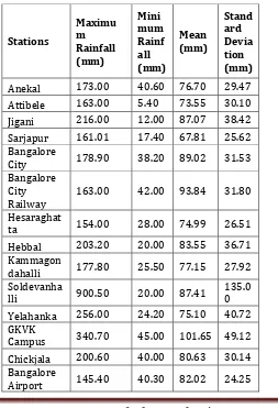
The daily 24 hour rainfall data for the years 1972 to 2011 was collected from IMD for 17 stations located in and around urban Bangalore. The 17 stations are Anekal, Attibele, Jigani, Sarjapura, Bangalore city, Bangalore city railway, Hesaraghatta, Hebbal, Kammagondahalli, Soldevanhally, Yelahanka, GKVK Campus, Chickjala, Bangalore Airport, Kengeri, Krishnarajapura and Tippagondanahalli. The stations considered had more than 75% of available raw data. The rest of the values had to be calculated. The missing rainfall values for the years 1972 to 2011 were calculated using normal ratio method, which is one of the most widely, used methods. The annual maximum 24 hour rainfall values were then extracted. The summary of statistics for peak daily rainfall is presented in table 1. The annual maximum 24 hour rainfall data extracted for 17 stations for the years 1972 to 2011 were used for the calculation of short duration rainfall using the IMD empirical reduction formula given in equation 3.2. Short duration rainfall depths were calculated for durations of 5, 10, 15, 30, 60, 120, 720 and 1440 minutes.

Table.1 statistics for peak daily rainfall

Stations

Maximu m Rainfall (mm)

Mini mum Rainf all (mm)

Mean (mm)

Stand ard Devia tion (mm) Anekal 173.00 40.60 76.70 29.47 Attibele 163.00 5.40 73.55 30.10 Jigani 216.00 12.00 87.07 38.42 Sarjapur 161.01 17.40 67.81 25.62 Bangalore

City 178.90 38.20 89.02 31.53 Bangalore

City

Railway 163.00 42.00 93.84 31.80 Hesaraghat

ta 154.00 28.00 74.99 26.51 Hebbal 203.20 20.00 83.55 36.71 Kammagon

dahalli 177.80 25.50 77.15 27.92 Soldevanha

lli 900.50 20.00 87.41 135.00 Yelahanka 256.00 24.20 75.10 40.72 GKVK

Campus 340.70 45.00 101.65 49.12 Chickjala 200.60 40.00 80.63 30.14 Bangalore

© 2017, IRJET | Impact Factor value: 5.181 | ISO 9001:2008 Certified Journal

| Page 1466

Krishnaraja

pura 236.40 9.80 66.59 47.04 Tippagonda

halli 395.84 35.36 69.88 55.09

The mean and standard deviations of the short duration rainfall depths were then calculated. These values were used in various probability distributions to find the rainfall depth and intensity. The mean and standard deviation extracted from short duration rainfall.

4.2 Rainfall depth and intensity

The short duration rainfall depths were calculated for the years 1972 to 2011 from IMD empirical reduction formula. Then the mean and standard deviations of short durations of 5, 10, 15, 30, 60, 120, 720 and 1440 minutes were estimated. These estimated mean and standard deviations were used in Normal, Log-Normal, Gumbel, Pearson, and Log-Pearson probability distribution methods to determine the rainfall depths and intensity for standard return periods of 2, 3, 5, 10, 25, 50, 100 and 200 years for 17 stations. It was found that the rainfall depths increased with the increasing time duration. But the rainfall intensity decreased appreciably with increasing duration. These distributions were subjected to chi-square goodness of fit test to find the best distribution.

4.2.1 Chi-square goodness of fit test

The rainfall depth and intensity for various short durations and standard return periods were found out using various probability distributions. These distributions were subjected to chi-square test to find the best distribution in which there is minimum deviation between the observed and the calculated value. It is found in the study that χ2 values for all probability distribution function, is increasing with increase in the rainfall duration. It is noticed that the Log-normal and Normal distribution shows the least deviations from the observed value. Normal distribution can also be considered as it is close to Log-normal distribution. But study showed that Log- Normal probability distribution function give the best estimation of the distributed predicted rainfall data as it has the smallest χ2 value compared to other distribution functions for the data collected for Urban Bangalore for the years 1972 to 2011. The other distributions are not consistent and show a huge deviation from the observed value.

4.2.2 IDF curve

It is noted from the IDF curves of that as the duration increases, the rainfall intensity decreases or in other words, for shorter duration the rainfall intensity is high.

Fig.2. IDF curve for Sodlvenahally

It was found from chi-square test that log-normal distribution gave the best results with minimum deviations from the observed values. Hence the IDF curve was plotted from log-normal values for each station considered.

5. CONCLUSIONS

Bangalore has emerged as industrial and commercial centre of India in recent times. Bangalore city in India has been subjected to intense urban growth and has led to sprawl. Due to this rapid urbanization as many as 70 per cent of the 262 water tanks in Bangalore have disappeared; drains are choked with garbage leading to surface flooding. Rapidly increasing human population coupled with the increased urban concentration has escalated both the frequency and severity of disasters like floods, etc. Some of the impacts due to urban development include: reclamation of lakes, stream widening and bank erosion, stream down cutting, changes in the channel bed due to sedimentation, increase in the floodplain elevation. Urban flooding is not a new phenomenon. Increasingly, more and more cities and towns face waterlogged streets. Development and redevelopment of the district, by nature increases the amount of imperviousness in the surrounding environment. This increased imperviousness translates into loss of natural areas, more sources for pollution in runoff, and heightened flooding risks. In recent decades, storm water runoff has emerged as an issue of major concern. Storm water affects local waterways both in terms of the volume of runoff that is generated, and the nature of the pollutants that may be conveyed. Allowing storm water to infiltrate in urban residential areas is one of the major ways for urban floods.

4.3 Scope for Future Work

© 2017, IRJET | Impact Factor value: 5.181 | ISO 9001:2008 Certified Journal

| Page 1467

weather conditions or long term climate cycles etc.

REFERENCES

[1] Bernard, M. M., (1932), “Formulas for rainfall

intensities of long durations”. Trans. ASCE 6:592 - 624.

[2] Central Water Commision, (2002), Training

module-12, “How to Analyse rainfall data”, http://www.cwc.gov.in/main/HP/download

[3] Chow V.T., D.R. Maidment and L.W.Mays, 1988,

“Applied Hydrology”, McGraw- Hill, Chapter 10 – Probability, Risk and Uncertainty Analysis for Hydrologic and Hydraulic Design: 361 – 398

[4] Eman Ahmed Hassan El-Sayed., (2011), “Generation of

Rainfall Intensity Duration Frequency Curves For Ungauged Sites”, Nile Basin Water Science & Engineering Journal,.4 (1): 112-124.

[5] Food and Agriculture Organization, (2012), Rainfall

Runoff Analysis, Rainfall Characteristics, http://www.fao.org/docrep/U3160E/u3160e05.htm

[6] Hershfield, D. M. (1961). Rainfall frequency atlas of

the United States for durations from 30 minutes to 24 hours and return periods from 1 to 100 years. U. S. D. o. C. Weather Bureau Technical Paper 40. Washington D.C.

[7] http://nptel.iitm.ac.in/courses/105108079/module6

/lecture24.pdf

[8] IDF-curve, (2012), IDF curve, what is an IDF curve?

http://www.idfcurve.org/default.aspx

[9] Indian Institute of Scienc, Centre for Ecological

Sciences, Energy and Wetlands research group, (2012), Study Area, Bangalore, Topography, Water Resources, and Meteorology, http://ces.iisc.ernet.in/energy/wetlands/sarea.html

[10] Indo-Asian News Service, (2013), Heavy rains lash

Bangalore, cripple normal life Karnataka, News - India Today.htm

[11] Kreyszig Erwin, (2006), “Advanced Engineering

Mathematics” Wiley John Wiley & Sons, Inc. Chapter 24 & 25 (991 – 1093)

[12] Kulkarni Vijay and Ramachandra T.V., 2006.

Environmental Management, Commonwealth Of Learning, Canada and Indian Institute of Science, Bangalore.

[13] Mohammadi Shirko Ebrahimi and Mahdavi

Mohammad, (2009), “Investigation of Depth-Area-Duration Curves for Kurdistan Province”, World Applied Sciences Journal 6 (12): 1705-1713

[14] National Programme on Technology Enchanced

Learning, Indian Institute of Technology, Madras, (2012), Stochastic Hydrology, Frequency Analysis, <http://nptel.iitm.ac.in/courses/105108079/module 6/lecture24.pdf> (Oct, 2012)

[15] Olofintoye, O.O, Sule, B.F and Salami, A.W., (2009),

“Best–fit Probability distribution model for peak daily rainfall of selected Cities in Nigeria”, New York Science Journal, 2(3):1-12

[16] Ramachandra T. V and Mujumdar Pradeep P. (2006),

“Urban Floods: Case Study of Bangalore”, Disaster &

Development Vol. 1 No. 2. Journal of the National Institute of Disaster Management.

[17] Rana Arun, (2011), “Avoiding natural disaster in

megacities – Case study for Urban Drainage of Mumbai”, Vatten 67:55–59.

[18] Rashid M. M., Faruque S. B and J. B. Alam, (2012),