REDUCTION OF MACHINING REJECTION OF SHIFT FORK BY USING
SEVEN QUALITY TOOLS
Akshay Jaware
1, Komal Bhandare
2, Gaurav Sonawane
3, Shraddha Bhagat
4, Rahul Ralebhat
51,2,3,4
Student of BE Mechanical, D. Y. Patil College Of Engineering, Pune, Maharashtra, India
[1],[2],[3]&[4]5
Professor, D. Y. Patil College Of Engineering, Pune, Maharashtra, India
[5]---***---Abstract -
In order to survive in a competitive market,improving quality and productivity of product or process is a must for any company. This study is about to apply the 7QC tools in the production processing line and on final product in order to reduce defects by identifying where the highest waste is occur at and to give suggestion for improvement. The approach used in this study is direct observation, thorough examination of production process lines, brain storming session, fishbone diagram, and information has been collected from potential customers and company’s workers through interview and questionnaire, Pareto chart/analysis, histogram and control chart was constructed. This paper intends to exhibit the exact application of seven quality tools in fork industry.
Key Words: Flow Chart, Pareto Chart, Scatter Diagram, Histogram, Cause & Effect Diagram, PP & Ppk , Why - Why Analysis, Hypothesis Test
1. INTRODUCTION
In today’s world, business has become more and more competitive. All industries and organizations have to perform well in order to survive and be profitable. “Quality” means those features of products which meet customer needs and thereby provide customer satisfaction. In this sense, the meaning of quality is oriented to income. The purpose of such higher quality is to provide greater customer satisfaction and, one hopes, to increase income. However, providing more and/or better quality features usually requires an investment and hence usually involves increases in costs. Higher quality in this sense usually “costs more.” One of the strongest motivating forces is "Delighted Customer". Industries believe that prosperity is directly linked with prosperity of customers. Mutual trust, healthy relationship, ethical values, innovative technologies, quality products and services are the constituents of commitment towards the customers. If defects are in large number it not only does an organization waste its resources and time to re-manufacture the products, but it also contributes to the loss of customers’ satisfaction and trust. Customer satisfaction comes from those features which induce customers to buy the product. Dissatisfaction has its origin in deficiencies and is why customers complain. Some products give little or no dissatisfaction; they do what the producer said they would do. Yet they are not saleable because some competing product has features that provide greater customer satisfaction. So it is important to reduce defects and maintain quality of product. Quality of the product is achieved by minimization of rework, reducing scrap rate and minimizing
man hour on rework. Now a day’s rework of rejected parts are common but rework add losses to the company net profit, if the company is a continuous mass production where the products go through a series of process to come out with final product. The Seven Quality Control Tools popularly called the 7 QC Tools, According to kaoru Ishikawa more than 95% company problems can be solved using these tools. It comprise of graphical methods and help to transform the data into easily understandable diagrams or charts. This further helps to understand the situation or to analyze the problem easily and leads to developing solutions which aim towards quality improvement. Further, these charts and diagrams help to highlight the important aspects of a problem clearly so that the concerned persons can focus attention on them and start developing the solution. Pareto analysis helps to identify and classify the defect according to percentage significant. Cause and effect diagram is a useful tool in identifying the major causes. This diagram helps to build a relationship. Brainstorming is done with utilizing these quality tools to provide an effective solution. Thus quality management tools are effective and significant in reducing the rework and rejection rate.
2. PROBLEM STATEMENT
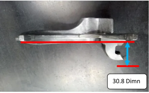
The rejection of shift fork 3rd 4th (S101) is very high due to machining defect of 30.8 dim not ok. Due to this variation in dimensions it cannot assembled in gearbox. About 313 no's job are rejected monthly at final inspection stage. So we lose productivity & face shortage in supply to customer.
Required size - 30.8 mm (variation +/- 0.12 mm is acceptable)
Maximum reading - 30.92 mm Minimum reading - 30.68 mm
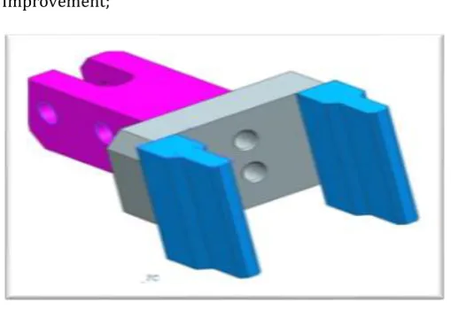
Fig -1: Defective Part
[image:1.595.311.558.616.770.2]3. OBJECTIVES
To increase productivity and profitability in an organization.
To reduce rejection rate of product.
To reduce rework and scrap of product.
To increase moral of internal customer of an organization.
To provide better solution for process improvement.
To get standardization for product using 7 QC tools.
To increase number of customer as getting high level of satisfaction of them including features like good design, value or price of product etc.
4. METHODOLOGY
The Seven Quality Control Tools popularly called the 7 QC Tools, comprise graphical methods and help to transform the data into easily understandable diagrams or charts. This further helps to understand the situation or to analyse the problem easily and leads to developing solutions which aim towards quality improvement. Further, these charts and diagrams help to highlight the important aspects of a problem clearly so that the concerned persons can focus attention on them and start developing the solution.
The 7 QC Tools listed in alphabetical order are:
1. Cause and Effect Diagram 2. Check sheet
3. Control Chart 4. Flow Chart 5. Histogram 6. Pareto chart 7. Scatter Diagram
These 7 QC tools can together enable a quality problem to be analysed and solved and also help to prevent a problem from recurring so that the quality problem is once for all solved. It is not the intention here to describe these tools in greater details as these tools are described in all quality related literature particularly textbooks and training manuals. It would not be exaggerating to say that almost all the quality control and management books include a description of the QC tools. Hence a detailed description can be found in many popular books, written by different authors, (Austrom & Lad, 1986), (Kume, 1987), (Chang, 1993), (Mears, 1994), (Wadsworth, Stephens, & Godfrey, 2001), (Evans & Lindsay, 2004), (Tague, 2005), (Defeo & Juran, 2010), and (Montgomery, 2012). As stated in
http://www.beyondlean.com/7-quality-tools.html, the 7 Quality Tools are problem solving tools which can:
• Help to identify and prioritize problems quickly and more effectively
• Assist the decision making process
• Provide simple but powerful tools for use in continuous improvement activity
• Provide a vehicle for communicating problems and resolution throughout the business
• Provide a way of extracting information from the data collected. To provide a continuity of reading a brief overview of all the seven tools is provided here.
Cause and Effect Diagram
The cause and effect diagram is also sometimes called as “fishbone diagram” or “Ishikawa diagram” after the Japanese quality expert late Dr. Kaoru Ishikawa. It is a useful method for listing and classifying the causes under different categories that lead to a problem or result or effect. The causes are classified according to their type or nature and represented in proper order.
The Diagram Consists of Two Sides
(1) Cause side – factors that influence the related effect or characteristic, and
(2) Effect side – represents a problem or an outcome in a given situation or a result. The two sides are connected by a thick arrow called the trunk. The arrow head leads to the effect side while branches and sub-branches added to the trunk represent the causes responsible for that effect. The major branches added to the trunk represent the main categories of causes and the small and tiny branches represent the sub-category of causes. The branches can be expanded or new branches can be introduced depending on the number of causes.
Check Sheet
A check sheet is a list in the form of a diagram or table format, prepared in advance to record data and is useful for later analysis. It is also called as a tally sheet. There are five basic types of check sheets as given below:
a) Classification -To classify the items under different headings
b) Location - To indicate position of an item
c) Frequency - To indicate the presence or absence of an item, and also the number of occurrences of that item d) Measurement scale - To provide a measurement scale divided into intervals to enable easy marking
e) Check list - To indicate the items or tasks to be performed to complete a task
Control Charts
A control chart is a line graph used to assess and validate the stability of a process. The graph consists of a horizontal center line and two parallel lines called upper control limit and lower control drawn on either side of the center line. Data pertaining to a quality characteristic is collected over a period of time and the values are plotted as points on the graph in the chronological order. The points are connected by straight lines.
control of the process. They also help in distinguishing the random causes from the assignable causes which need to be investigated further. When all the points are within the control limits, and these points do not exhibit any abnormal pattern, then the underlying process is said to be under statistical control. In such cases no action may be necessary and the process is allowed to continue. If the points fall outside the control limits or display any abnormal pattern, then the process is deemed to be out of control and under the influence of special causes. In such cases the process would be stopped and investigated for causes. Then the required corrective action is taken and the process is continued. The control charts used in industries are divided into two groups namely Control charts for variables, and Control charts for attributes.
Flow Chart
A flowchart is a graphical method of displaying a system’s operation or sequence. A familiar type of flowchart is the computer program flowchart, which is used in programming. A flowchart consists of several standard symbols connected in a logical manner to depict the flow of operations or information or tasks in the desired sequence.
Histogram
A histogram is a frequency distribution diagram which displays the distribution of data in the form of a bar graph. It is constructed from the data collected in a frequency table which shows the data distributed across several class intervals and the frequency of occurrence under each class. The histogram drawn from the frequency table is composed of columns whose widths represent the class interval and the height represents the frequency. The histogram provides a visual representation of the data distribution and gives a quick assessment on the spread and shape of the distribution.
Pareto Diagrams
A Pareto diagram, named after Vilfredo Pareto, an Italian economist, is a specialized bar graph that can be used to show the relative frequency of events such as defects, repairs, claims, failures, or any other entity, in the descending order. This helps to focus on the vital few and not to start with the trivial many, to improve the quality.
Scatter Diagram
A scatter diagram represents the relationship between two types of data or two variables. The two variables are plotted along the two conventional coordinate axes and the relationship between the variables will be evident by the scatter or spread of the points. Thus a scatter diagram helps to find the correlation between two variables.
5. LITERATURE REVIEW
The key to the vast storehouse of published literature may open doors to sources of significant problems and
explanatory hypothesis and provide helpful orientation for definition of the problem, background for selection of procedure and comparative data for interpretation of results. In order to be creative and original one must read extensively and critically as a stimulus to thinking. Every research begins from where the previous researches have left it, and goes forward, may be one inch or even less, towards finding the solution of a problem or answer to a question.
Chiragkumar S. Chauhan et al (2013) this article states that Quality tools can be used in all phases of production process, from the beginning of product development up to product marketing and customer support. Once the quality improvement process is understood, the addition of quality tools can make the process proceed in a systematic manner. Many quality tools are available for quality professionals for this purpose. Many organizations use total quality management (TQM) tools to identify, analyze and assess qualitative and quantitative data that are relevant to their processes. The flowchart is simply a visual description of a process. A cause-and-effect diagram is a brainstorming-based problem-solving procedure. Check sheets and Pareto diagrams are simply common sense tools. Histograms scatter diagrams, and control charts are the only statistical tools in the list. The key to their success in problem-solving and process improvement initiatives are their simplicity, ease of use and their graphical nature. They can easily be taught to any member of the organization. In the paper the systematic approach to the quality improvement is shown on the simple example of a company in process industry. The company defined the principle of quality management as basic principle with goals of continuous improvement. Customer satisfaction is placed on the top of value scale, while data analysis is conducted permanently in order to recognize opportunities for process quality improvement. Selected company from process industry has certified quality management system in accordance with ISO 9000:2000. Company that manage its quality system in accordance with ISO 9000:2000 has to plan and implement process control, measurement, analysis and improvement in order to: Demonstrate conformity of its products, achieve conformity of its quality management system, continuously improve efficiency of its quality management system. The number of customer claims is collected for three consecutive business years. On the end of each business year customer claims are systematically analyzed in order to identify type and amount of customer claims for year in consideration. Also, the undertaken corrective and preventive actions are analyzed to verify their effectiveness. One of broadly used tools to visualized collected data is histogram. Other 7QC tools are used in order to evaluate is there more opportunities to improve process and meet customer demands. Research has been conducted in order to define role and importance of seven basic quality tools (7QC tools) within quality management system. In modern production processes it is necessary to implement integrated quality management system that involves quality management, responsible environmental performance and safe working environment. Systematic application of 7QC tools will enable successful quality improvement process. Quality tools has important place in data collecting, analyzing, visualizing and making sound base for data founded decision making. The paper stresses on the use of the seven basic quality tools to improve processes and to solve problems.
Kirti Singh et al (2016) The study exhibited in this chapter includes simple approach in the analysis of rejection rate in particular production line in gloves manufacturing shop. The production line consists of sequence of operation in making final product. Defects occur due to deficiency in manufacturing process. The study aims at analyzing the
rework, man hour spent on rework and taking effective measures will enhance the net profit, saves time and improve overall quality of product.
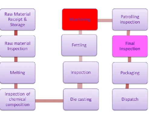
6. PROCESS FLOW DIAGRAM
[image:5.595.308.559.75.258.2]
Fig -2: Process Flow Diagram
Problem generated at machining stage and detected at final inspection stage.
7. DATA COLLECTION AND ANALYSIS
Data collected consist of mainly defects that occur in a manufacturing of fork. But our area of interest is the defects causing at machining process. The defects causing rejection of product from the production process were identified from the data. To identify main problems which cause frequent defects of fork production, a six month data had been collected(July to December 2017). The actual rejection is grouped in their respective type of defect identified.
Table -1: Data of six months
Defects Total Total
Sum Rej% Cum Rej
30.8 Dimn not
ok 1201 1513 79.38 79.38
Non filling 188 1513 12.43 91.80
G not ok 70 1513 4.63 96.43
Blow Hole 21 1513 1.39 97.82
Patch mark 17 1513 1.12 98.94
Dent/Damage 13 1513 0.86 99.80
Crack 2 1513 0.13 99.93
Bush crack 1 1513 0.07 100.00
7.1 Pareto Chart
Pareto chart is constructed based on data collected and to identify most common defects.
Chart -1: Pareto Chart
Pareto chart revealed that 2.9% constitutes of other defects, 3.7% G not ok, 10% is of non filling and 83.4% is of 30.8 dimn not ok.
Only the major defect identified is chosen for analysis. According to pareto, 80-20 rule we have to need take action for 30.8 dimn not ok.
7.2 A REAL TIME 4M CONDITIONS
[image:5.595.38.285.133.321.2]4M consists of man, machines, material and method.
Table -2: 4M Conditions
4M condition
Control items (Managing
points ) Specification Observation
Current status
Machine
Clamp condition of
fixture
After clamping
clamp should not
be loose
found one clamp loose
after clamping
the job
ok
Coolant
concentration 4-6 % 1.60% x
Clamp
pressure 25-35 Kg/ Cm² 31 Kg/ Cm² ok
Method
Tool life
As per tool life defined monitoring
sheet
Tool life not Monitored x
Insert wear
out No wear out
Built up edge wear
not found on tool
ok
Wrong Gauge calibrated should be calibrated Gauge is ok
Material composition Metal drawing As per
As per drawing
found within spec
ok
Man unskilled operator
/inspector skill matrix
As per skill matrix, found semi
skilled
ok
Current status: O - Ok for 4M condition X - Not ok for 4M condition
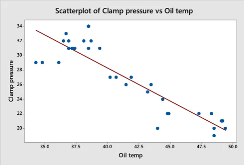
7.3 SCATTER DIAGRAM
The data of oil temperature and clamping pressure is collected time to time and scatter diagram is plotted.
50.0 47.5 45.0 42.5 40.0 37.5 35.0 34
32
30
28
26
24
22
20
Oil temp
C
la
m
p
pr
es
su
re
[image:6.595.30.566.38.815.2]Scatterplot of Clamp pressure vs Oil temp
Fig -3: Scatter Diagram
From above scatter plot we get that lubricate oil temp increased then clamping pressure is to be decreased so there is negative correlation.
8. ANALYSIS
Table -3: Measurements of 50 no’s of samples
Sr
No knesThic s at A
Thickne
ss at B Variation A to B
Thickne
ss at C Variation A to C
1 7.04 7.03 0.01 7.1 -0.06
2 7.04 7.03 0.01 7.04 0
3 7.02 7.03 -0.01 7.05 -0.03
4 7.05 7.04 0.01 7.1 -0.05
5 7.04 7.04 0 7.08 -0.04
6 7.04 7.03 0.01 7.06 -0.02
7 7.05 7.05 0 7.09 -0.04
8 7.03 7.03 0 7.04 -0.01
9 7.03 7.03 0 7.06 -0.03
10 7.04 7.04 0 7.04 0
11 7.02 7.02 0 7.03 -0.01
12 7.05 7.04 0.01 7.07 0.02
13 7.04 7.05 -0.01 7.1 -0.06
14 7.04 7.05 -0.01 7.07 -0.03
15 7.03 7.04 -0.01 7.06 -0.03
16 7.05 7.04 0.01 7.09 -0.04
17 7.04 7.05 -0.01 7.08 -0.04
18 7.05 7.06 -0.01 7.1 -0.05
19 7.02 7.03 -0.01 7.07 -0.05
20 7.05 7.04 0.01 7.07 -0.02
21 7.03 7.04 -0.01 7.04 -0.01
22 7.03 7.03 0 7.05 -0.02
23 7.04 7.03 0.01 7.1 0.06
24 7.03 7.04 -0.01 7.05 -0.02
25 7.04 7.05 -0.01 7.09 -0.05
26 7.03 7.03 0 7.07 -0.04
27 7.04 7.04 0 7.08 -0.04
28 7.05 7.04 0.01 7.08 -0.03
29 7.04 7.05 -0.01 7.09 -0.05
30 7.03 7.04 -0.01 7.06 -0.03
31 7.04 7.03 0.01 7.05 -0.01
32 7.04 7.05 -0.01 7.08 -0.04
33 7.04 7.04 0 7.08 -0.04
34 7.05 7.05 0 7.09 -0.04
35 7.04 7.04 0 7.08 -0.04
36 7.03 7.04 -0.01 7.06 -0.03
37 7.03 7.04 -0.01 7.07 -0.04
38 7.04 7.05 -0.01 7.1 -0.06
39 7.04 7.06 -0.02 7.09 -0.05
40 7.03 7.03 0 7.08 -0.05
41 7.03 7.04 -0.01 7.08 -0.05
42 7.02 7.03 -0.01 7.09 -0.07
43 7.02 7.03 -0.01 7.02 0
44 7.05 7.05 0 7.1 -0.05
45 7.04 7.03 0.01 7.08 -0.04
46 7.03 7.04 -0.01 7.06 -0.03
47 7.05 7.06 -0.01 7.09 -0.04
48 7.02 7.02 0 7.09 -0.07
49 7.03 7.04 -0.01 7.09 -0.06
50 7.05 7.05 0 7.04 0.01
Fig -4: Positioning of fork on fixture
A
[image:6.595.36.282.230.396.2]Fig -5: Thickness of resting pad
7.06 7.05
7.04 7.03
7.02 20
15
10
5
0
Mean 7.037 StDev 0.009530 N 50
Thickness at A
Fr
eq
ue
nc
y
[image:7.595.42.294.62.457.2]Histogram of Thickness at A Normal
Fig -6: Histogram of A
Calculation
Mean = 7.037
Standard deviation (𝜎) = 0.00953 USL = 7.1
LSL = 6.9
Range (R) = Xmax - Xmin = 7.05 – 7.02
= 0.03
Average (X) = 7.037 PP =
= (7.1 – 6.9)/6 * 0.00953 = 3.4977
PpU =
= (7.1 – 7.037)/3 * 0.00953 = 2.2035
PpL =
= (7.037 – 6.9)/3 * 0.00953 =4.791
Ppk = 2.2035
(Ppk ≥ 1.67 is desirable)
7.06 7.05 7.04 7.03 7.02 20
15
10
5
0
Mean 7.040 StDev 0.009681
N 50
Thickness at B
Fr
eq
ue
nc
y
Histogram of Thickness at B
Normal
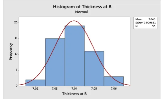
Fig -7: Histogram of B
Calculation
Mean = 7.04
Standard deviation (𝜎) = 0.009681 USL = 7.1
LSL = 6.9
Range (R) = Xmax - Xmin = 7.06 – 7.02
= 0.04
Average (X) = 7.0396 PP =
= (7.1 – 6.9)/6 * 0.009681 = 3.4431
PpU =
= (7.1 – 7.0396)/3 * 0.009681 = 2.0796
PpL =
= (7.037 – 6.9)/3 * 0.009681 =4.8066
Ppk = 2.0796
(Ppk ≥ 1.67 is desirable)
7.12 7.10 7.08 7.06 7.04 7.02 10
8
6
4
2
0
Mean 7.073 StDev 0.02107
N 50
Thickness at C
Fr
eq
ue
nc
y
Histogram of Thickness at C
[image:7.595.303.561.74.232.2]Normal
Fig -8: Histogram of C Calculation
Mean = 7.073
[image:7.595.309.561.553.706.2]LSL = 6.9
Range (R) = Xmax - Xmin = 7.1 – 7.01
= 0.09
Average (X) = 7.0726 PP =
= (7.1 – 6.9)/6 * 0.02107 = 1.5820
PpU =
= (7.1 – 7.037)/3 * 0.02107 = 0.4334
PpL =
= (7.037 – 6.9)/3 * 0.02107 =2.7305
Ppk = 0.4334
(Ppk ≥ 1.67 is desirable)
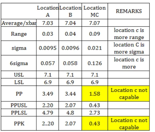
[image:8.595.306.562.214.418.2]At location ‘C’ pp & ppk ≤1.67 so location
c is only creating
the problem
.Table -4: Result table
Location
A Location B Location MC REMARKS Average/xbar 7.03 7.04 7.07
Range 0.03 0.04 0.09 location c is more range
sigma 0.0095 0.0096 0.021 location C is more sigma
6sigma 0.057 0.058 0.126 location c is more
USL 7.1 7.1 7.1
LSL 6.9 6.9 6.9
PP 3.49 3.44 1.58 Location c not capable
PPUSL 2.20 2.07 0.43
PPLSL 4.79 4.8 2.73
PPK 2..20 2.07 0.43 Location c not capable
[image:8.595.36.298.345.567.2]9. CAUSE & EFFECT DIAGRAM
Fig -9: Cause And Effect Diagram
Probable causes for thickness variation at location “C”
1. warpage in casting at location “c”. 2. Fixture rest pad plane variation. 3. In adequate clamping.
4. Clamping pressure variation is already concluded in quick win solution.
[image:8.595.36.544.412.765.2]10. HYPOTHESIS TEST
Table -5: Hypothesis
Sr No PROBABLE CAUSES OBSERVATIONS TESTING & CONCLUSION
1 CASTING BEND
50 NOS NOT OK PART AS CAST BEND CHECK
FOUND ALL ARE WITHIN SPEC
Hypothesis invalid
2 REST PAD FIXTURE VARIATION
ALL REST PAD CHECKED AND FOUND
DIFFERENCE WITHIN 0.010 MM AS PER SPEC
Hypothesis invalid
3 ADIQUATE IN CLAMPING
AFTER CLAMPING PLAY OBSERVED AT LOCATION "C" UPTO 0.50 TO 1.0MM ( CHECKED BY DIAL
GAUGE )
Hypothesis valid
From above we found in adequate clamping is the valid probable cause.
11. WHY - WHY ANALYSIS
Chart -2: Analysis Flow Chart Inadequate clamping
Why
Play after clamping
Clamp not resting on part
Why
Why
Variation in part height (at location
“A” &“C”
Clamp not able to accommodate casting
12. ACTION
Immediate Action
Coolant concentration checking & monitoring started by refractory meter shift wise (specification - 4-5 %)
[image:9.595.50.561.98.830.2]Tool change frequency set (25,000 ) and started monitoring.
Table -6: Root Cause Analysis
Root causes Action plan Remarks
variation in part height (at
location “a” & “c”
casting height is to be maintain at same level by
modifying part design
not possible due to design
constant
clamp not able to accommodate casting height
variation
single part machining at a
time in single fixture productivity low
individual clamp is to be used for individual part
not feasible due to space
constant in fixture clamp design is to be
modify to accumulate
casting height variation ok
Actions Decided
Table -7: Action Planning
Root
Cause Action Plan Target Date Actual Date Status
Clamp not able to accommo date casting height variation
Clamp design is to be modify to accumulate casting height variation
25.03.18 18.04.18 close
13. RESULTS
7.06 7.05 7.04 7.03 7.02 7.01 18
16
14
12
10
8
6
4
2
0
Mean 7.038 StDev 0.01212
N 50
Thickness at A
Fr
eq
ue
nc
y
Histogram of Thickness at A
Normal
Fig -10: Histogram of A
PP = 2.75027 Ppk = 1.70517
(Ppk ≥ 1.67 is desirable)
7.05 7.04
7.03 7.02
20
15
10
5
0
Mean 7.035 StDev 0.01015 N 50
Thickness at B
Fr
eq
ue
nc
y
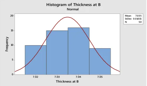
Histogram of Thickness at B Normal
[image:9.595.308.560.123.270.2]
Fig -11: Histogram of B
PP = 3.28407 Ppk = 2.14121
(Ppk ≥ 1.67 is desirable)
7.06 7.05
7.04 7.03
7.02 7.01
20
15
10
5
0
Mean 7.035 StDev 0.01054 N 50
Thickness at C
Fr
eq
ue
nc
y
Histogram of Thickness at C
Normal
Fig -12: Histogram of C
PP =3.16255 Ppk = 2.06198
(Ppk ≥ 1.67 is desirable)
Table -8: Final Result Table
Location
A Location B Location MC Remarks Average/xbar 7.038 7.034 7.034
Range 0.04 0.03 0.03
sigma 0.0121 0.0101 0.0105 6sigma 0.072 0.06 0.063
USL 7.1 7.1 7.1
LSL 6.9 6.9 6.9
PP 2.75 3.28 3.16 Location “c” is capable
PPUSL 1.70 2.14 2.06
PPLSL 3.79 4.42 4.26
From the table we see that pp & ppk ≥1.67 in all locations so action is effective.
1st Quartile 7.0600 Median 7.0800 3rd Quartile 7.0900 Maximum 7.1000
7.0666 7.0786
7.0700 7.0800
0.0176 0.0263 A-Squared 1.23 P-Value <0.005
Mean 7.0726
StDev 0.0211
Variance 0.0004 Skewness -0.576058 Kurtosis -0.540079
N 50
Minimum 7.0200 Anderson-Darling Normality Test
95% Confidence Interval for Mean
95% Confidence Interval for Median
95% Confidence Interval for StDev 7.10
7.08 7.06 7.04 7.02
Median Mean
7.0800 7.0775 7.0750 7.0725 7.0700 7.0675 7.0650
95% Confidence Intervals
Summary Report for Before action
[image:10.595.35.282.110.367.2]
Fig -13: Summary report before action
1st Quartile 7.0300 Median 7.0350 3rd Quartile 7.0400 Maximum 7.0500
7.0318 7.0378
7.0300 7.0400
0.0088 0.0131 A-Squared 2.23 P-Value <0.005
Mean 7.0348
StDev 0.0105
Variance 0.0001 Skewness 0.00035 Kurtosis -1.17757
N 50
Minimum 7.0200 Anderson-Darling Normality Test
95% Confidence Interval for Mean
95% Confidence Interval for Median
95% Confidence Interval for StDev 7.05
7.04 7.03 7.02
Median Mean
7.040 7.038 7.036 7.034 7.032 7.030
95% Confidence Intervals
Summary Report for After action
Fig -14: Summary report after action
Both data are not normal as p value is < 0.05
Null hypothesis (Ho); sigma A = sigma B
Alternative hypothesis (Ha); sigma A is significantly different from sigma B
.
Here p value is ≤0.05 so we reject Ho & Accept Ha i.e. The variation After action is significantly improved from Before action
.
After action Before action
7.10
7.09
7.08
7.07
7.06
7.05
7.04
7.03
7.02
7.01
D
at
a
Individual Value Plot of Before action, After action
[image:10.595.36.288.406.663.2]
Fig -15: Individual Value plot Before & After Action
This graph cleared that thickness variation after action is significantly improved then before action.
Chart -3: Bar Graph of Effectiveness of Actions
After action taken % rejection reduced to 0.65 % from average16.66 % before project.
Production loss reduced from 262 no’s per month to 51 no’s per month (Rejection reduced 211 no’s/per month).
[image:11.595.35.290.370.545.2]13.1 BENEFITS AND IMPROVEMENT
Table -9: Direct Benefits
Cost Details Project Before Project After Rs per annum Cost saving in Avg Number of
pieces scrapped per
month 262 51
cost of scraped per
month 31440 6120
saving in cost per
year 303840
Intangible benefits
;
1. Customer demands are fulfilled. 2. Increase productivity.
3. Increase in employee’s moral. 4. Cost of poor quality decreased.
Improvement;
Fig -16: Clamp Before Status
As clamp is bolted in 2 positions there is no scope for adjustment for variable height of 2 different forks.
Fig -17: Clamp After Status
As clamp is bolted in 1 position there is scope for adjustment for variable height of 2 different forks as it allows clamp to float.
14. CONCLUSION
Quality leads to improvement in productivity and at the same time it also leads to customer’s satisfaction. Study has been conducted to define the role of quality control tools in fork manufacturing industry. Quality tools are not so wider spread as expected although they are quite simple for application and easy for interpretations. Main goal of the study is to reduce the cost per component by reduction in monthly rejection of the components After studying the problems, various parameters affecting the quality of the final product were identified and data was collected with accuracy and precision. Most of the quality tools are used in the study. The main conclusions of the study are summarized as below.
Fixture design validation is to be done during process designing & approval.
Rejection of the fork has been reduced from 16.66% to0.65% for overall production of components.
Saving of Rs. 3.03 lakhs per year.
Process is standardized and additional audit is started.
REFERENCES:
[1] Varsha M. Magar1, Dr. Vilas B. Shinde, “Application of 7
Quality Control (7 QC) Tools for Continuous Improvement of Manufacturing Processes,” International Journal of Engineering Research and General Science Volume 2, Issue 4, June-July, 2014, ISSN 2091-2730
[2] Chiragkumar S. Chauhan1 Sanjay C. Shah2 Shrikant P.
Bhatagalikar3, “Quality Improvement By Apply Seven Quality Control (7 QC) Tool in Process Industry,” IJSRD - International Journal for Scientific Research & Development| Vol. 1, Issue 10, 2013 | ISSN (online): 2321-0613
[3] Kirti Singh, Avinash Nath Tiwari, “Defects Reduction
Using Root Cause Analysis Approach in Gloves Manufacturing Unit,” International Research Journal of Engineering and Technology (IRJET), Volume: 03 Issue: 07 | July -2016
[4] Deepak1, Dheeraj Dhingra2, “APPLICATION OF QUALITY
CONTROL TOOLS IN A BICYCLE INDUSTRY: A CASE STUDY,” IJRET: International Journal of Research in Engineering and Technology
[5] 1Shyam H. Bambharoliya, 2Hemant R. Thakkar,
[6] Milind Raut, Dr. Devendra S. Verma, “To Improve Quality
and Reduce Rejection Level through Quality Control,” International Journal on Recent and Innovation Trends in Computing and Communication, ISSN: 2321-8169Volume: 5 Issue: 7
[7] Yonatan Mengesha Awaj, Ajit Pal Singh1, Wassihun
Yimer Amedie, “QUALITY IMPROVEMENT USING STATISTICAL PROCESS CONTROL TOOLS IN GLASS BOTTLES MANUFACTURING COMPANY,” International Journal for Quality Research 7(1) 107–126, ISSN 1800-6450
[8] Sulaman Muhammad, “Quality Improvement Of Fan
Manufacturing Industry By Using Basic Seven Tools Of Quality: A Case Study,” Sulaman Muhammad Int. Journal of Engineering Research and Applications www.ijera.com ISSN : 22489622, Vol. 5, Issue 4, ( Part -4) April 2015, pp.30-35
[9] Duško Pavletić, Mirko Soković, Glorija Paliska, “Practical
Application of Quality Tools,” International Journal for Quality research, UDK- 658.562
[10] Petruta Blaga, Boer Jozsef, “The influence of quality tools
in human resources management,” Procedia Economics and Finance 3 ( 2012 ) 672 – 680
[11] Amir Azizi, “Evaluation Improvement of Production
Productivity Performance using Statistical Process Control, Overall Equipment Efficiency, and Autonomous Maintenance,” 2nd International Materials, Industrial, and Manufacturing Engineering Conference, MIMEC2015, 4-6 February 2015, Bali Indonesia
BIOGRAPHIES
“Akshay Jaware Studying in B.E. Mechanical D Y Patil College of Engineering, Pune, Maharashtra, India”
“Komal Bhandare Studying in B.E. Mechanical D Y Patil College of Engineering, Pune, Maharashtra, India”
“Gaurav Sonawane Studying in B.E. Mechanical D Y Patil College of Engineering, Pune, Maharashtra, India”
“Shraddha Bhagat Studying in B.E. Mechanical D Y Patil College of Engineering, Pune, Maharashtra, India”
“Rahul Ralebhat Professor at D Y Patil College of Engineering, Pune, Maharashtra, India”