Recent Trends in 2d to 3d Image Conversion: Algorithms at a glance

(1)

RECENT TRENDS IN 2D TO 3D IMAGE CONVERSION:

Algorithms at a glance

Avi Kanchan

1

_{, Tanya Mathur}

2

1

_{Student, Department of Computer Science Engineering, KIET, Ghaziabad, India}

2

_{Asst. Professor, Department of Computer Science Engineering, KIET, Ghaziabad, India}

---*---Abstract -**

We present a paper on state of the art methods

of 2D to 3D image conversion. In this modern era, 3D contents are dominated by its 2D counterpart. Today there exists an urgent need to convert the existing 2D content to 3D. Mainly, these conversion methods are categorised in an automatic method and semi-automatic method. In an automatic method, human intervention is not involved, whereas in semi-automatic method human operator is involved. The main difference between 2D and 3D images is clearly the presence of depth in 3D images which makes the calculation of depth the most important factor. Until now many researchers have proposed different methods to close this gap. This paper describes and analyses algorithm that uses monocular depth cues and by learning depth from examples, establishing an overview and evaluating its relative position in the field of conversion algorithms. This may, therefore, contribute to the development of novel depth cues and help to build better algorithms using combined depth cues.

1. INTRODUCTION

We must begin our journey by taking issue with the philosophical adage that "a picture is worth a thousand words." It is my belief that a picture cannot begin to convey the depth of human experience and wisdom embedded in the words of Shakespeare. Nonetheless, pictures do contain a wealth of information and have been used throughout the centuries as an important and useful means of communication. An image is a picture representing visual information. A 2D image has only two dimensions height and width, while in a 3D image along with height and width it contains a third parameter called depth. The 3D image provides more information and gives better real-time world experience than 2D image. The advent of innovative 3D technology and

accruing sales of 3D consumer electronics have accompanied an increase in demands of more and more 3D technology. Despite the advent of 3D technology, the availability of 3D content is still hindered by that of its 2D correspondent. To close this gap, many 2D-to-3D image conversion methods have been proposed. Two approaches to 2D to 3D conversion can be loosely defined: semi-automatic conversion and automatic conversion. In semi-automatic conversion, a skilled operator assigns depth to various parts of an image or video. In automatic methods, operator interference is not required despite a computer algorithm automatically measures the depth for a single image. Automatic methods estimate shape from shading, structure

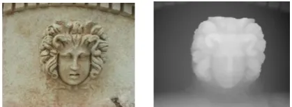
from motion or depth from defocus. , have not yet achieved the same level of quality for they rely on assumptions that are often violated in practice. Methods involving human operators have been most successful but also time-consuming and costly. The main difference between 2D and 3D images is clearly the presence of depth in 3D images which makes the calculation of depth the most important factor in the conversion of images from 2D to 3D. There are two steps in 2D to 3D conversion process: depth estimation for a given 2D image and depth-based rendering of a new image in order to form a stereo pair. While the rendering step is well understood and algorithms exist that produce good quality images, the main problem is in estimating depth from a single image. Several methods have been proposed for the same. Out of these, we shall study mainly two methods. First, calculating the depth using monocular depth cues and then by learning depth via a simplified algorithm that learns the scene depth from a large database which is having an image and depth pairs. To compare these two methods, we use the generation of a depth map. A depth map is a 2D function that gives the depth (with respect to the viewpoint) of an object point as a function of the image coordinates. The depth map is a kind of image which is composed of the gray pixels defined by 0 ~ 255 values. The "0" value of gray pixels stand for that "3D" pixels are located at the most distant place in the 3D scene while the "255" value of gray pixels stand for that "3D" pixels are located at the most near the place. In-depth map, each depth pixel would define the position in Z-axis where its corresponding 2D pixel will be located. It is called as pixel-by-pixel which produces a reasonably good 3D image, it is now widely used for producing 3D contents, especially the multi-view 3D contents for 3D digital signage.

[image:1.595.329.539.604.681.2]

Figure 1: A 2D image and its depth map

2.

ESTIMATING DEPTH BY LEARNING DEPTH FROM

EXAMPLES

(2)

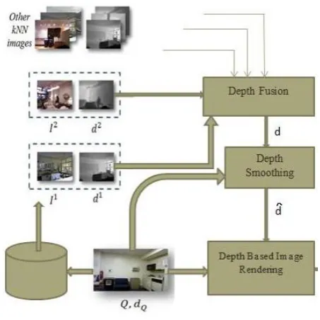
[image:2.595.37.264.419.645.2]

In this method, a simplified algorithm [1] is proposed that determines the depth of the scene from a huge database which contains image and depth pairs. Such methods can generate depth maps for any 2D visual material but currently, work on only a few types of images using carefully selected training data is done. They are computationally more efficient than the other algorithms. Their projected method is situated on the scrutiny that there are probably many pairs whose 3D content is similar to that of a 2D input. Also, they have made two assumptions that two images that are photometrically similar are likely to have similar 3D structure i.e. depth [2].Since photometric properties are often correlated with 3D content as depth, disparity. For example, edges of a depth map almost always coincide with photometric edges. Figure 2 shows the block diagram of our approach. The sections below provides a description of each step. In these sections, Q is the query image for which a right image QR is being sought. We assume that a database I = {(I1, d1), (I2, d2), ...} of image + depth pairs (I k, d k ) is available. Note that a database of stereoscopic images could be processed to extract image + depth pairs. The goal is to find a depth estimate ^ d and then a right image estimate ^QR given the 3D database I.

Figure 2: Block diagram of the overall algorithm:

Step 1: kNN Search

There are two types of images in a 3D image repository: those which are relevant for determining depth from a 2D query image, and those which are irrelevant. Images that are photometrically different to the 2D query are dejected because they are incompetent in the depth estimation process. Choosing a smaller subset of images gives an added advantage practically of computational tractability when the dictionary size is very large.

Our 2D query image Q is the left image from a stereo pair whose right image QR is unknown. We assume that a database of 3D images such as the NYU depth database, is available and that for each RGB image Ii in the database the corresponding depth field di is either known or can be computed from a stereo pair One method for selecting a useful subset of depth relevant images from a large image dictionary is to select only the ‘k' images that are closest to the input where closeness is measured by some distance function which captures global image properties such as color, texture, edges, etc. For the distance function, we use the Euclidean norm of the difference between histograms of oriented gradients (HOGs) computed from two images. Each HOG comprises of 144 real values (4×4 blocks with 9 gradient direction bins) which can be efficiently computed. This image closeness measure is significantly less complex computationally as compared to the weighted Hamming distance between the binary hashes of features used originally.

We perform a search for the top matches to our 2D query among all the 3D images in the database I, which search returns an ordered list of image + depth pairs, from the most to the least photometrically similar ones to the 2D query. We discard all matches except the top ‘k' ones (kNNs) from this list.

Step 2: Depth Fusion

None of the NN image + depth pairs (Ii_{, d}i_{), i ∈ K may match a}

query Q accurately. If a similar object (e.g., table) appears at a similar location in several kNN images, then such an object can also appear in the query and the depth field being sought should reflect this. This depth field is ciphered by using the median operation on the kNN depths at each dimensional location x as follows:

d[x] = median{di_{[x], ∀ i ∈ K}.}

Although these depths are overly smooth, they provide a globally correct, although coarse, assignment of distances to various areas of the scene.

Step 3: Cross Bilateral Filtering

Although median-based fusion helps in making depth globally consistent, the fused depth hence developed is locally inconsistent and very smooth due to the following reasons:

1. Misalignment of edges between the fused depth field and query image,

2. Lack of fused depth edges where sharp object boundaries occur,

3. Lack of fused depth smoothness where smooth depth changes are expected.

(3)

hσ (x) = exp (−_x_2/2σ2)/2πσ2 is a Gaussian weighting

function. Note that the directional smoothing of d is controlled by the query image via the weight hσe (Q[x] −

Q[y]). For large discontinuities in Q, the weight hσe (Q[x] −

Q[y]) is small and thus the contribution of d[y] to the output is small. However, when Q[y] is similar to Q[x] then hσe (Q[x] − Q[y]) is relatively large and the contribution of d[y] to the output is larger. In essence, depth filtering (smoothing) is happening along (and not across) query edges. The filtered depth preserves the global properties captured by the unfiltered depth field d and is smooth within objects and in the background. At the same time, it keeps edges sharp and aligned with the query image structure.

Step 4: Stereo Rendering

In order to generate an estimate of the right image _ QR from the 2D query Q, we need to compute the disparity δ from the estimated depth _ d. Let us suppose that a parallel camera with focal length f and baseline B captures a fictitious image pair (Q,_QR), the disparity comes out to be δ[x, y] = Bf/_d[x], where x = [x, y]T_{. We forward-project the 2D query Q to}

produce the right image:

while rounding the location coordinates (x + δ[x, y], y) to the nearest sampling grid point. We handle occlusions by depth ordering: if (xi + δ[xi, yi], yi) = (xj + δ[xj, yi], yi) for some i, j, we

assign to the location (xi + δ[xi, yi], yi) in QR an RGB value

from that location (xi, yi) in Q whose disparity δ[xi, yi] is the

largest. In newly-exposed areas, i.e., for xj such that no xi

satisfies (xj, yi) = (xi + δ[xi, yi], yi), we apply simple in painting

using in paint nans from Matlab Central.

3. ESTIMATING DEPTH BY USE OF MONOCULAR

DEPTH CUES

[image:3.595.310.512.113.246.2]

An automatic algorithm for 2D to 3D conversion is based on multiple depth cues, the three depth cues considered here are perspective geometry, defocus, visual saliency and adaptive depth models [3]. Three distinct depth generation procedures have been considered along with appropriate 2D scene features, a single depth generation procedure is performed. Figure 3 shows proposed an algorithm for conversion. Before starting this algorithm flow as shown in figure 3, the first colour image is converted into a grayscale image. This grayscale image is then given to the flow.

Figure 3: diagram of point transformation in

(4)

4.

FUTURE WORK

It can be observed that a lot of the 2D to 3D conversion algorithms are still in the research phase. The factors such as unsatisfactory quality and high complexity make it inadequate for real time use. As well as improving the existing algorithms, a new trend in this field is to analyse the semantic content of the image and use this knowledge to help reconstruct the 3D object. The depth cue “statistical patterns” plays the central part in this trend. The recently developed algorithm of Battiato [6] et al. using the image classification technique. The algorithm operates on a single colour image. A prior knowledge of the image content is needed. It is also claimed to be fully unsupervised and suitable for real-time applications. Eight steps [9] are involved in this algorithm. In this algorithm, two depth maps are constructed namely, the geometric depth map and the qualitative depth map.In the end, these two depth maps are combined together to generate the final depth map. The steps are:

1. Color-based segmentation.

2. Rule-based regions diction to find specific areas. 3. Qualitative depth map construction.

4. In order to distinguish images are classified into: Indoor, Outdoor without geometric appearance, Outdoor with geometric appearance.

5. Vanishing lines detection.

6. Geometric depth map construction.

7. Consistency verification of detected regions.

8. Amalgamation of the qualitative and the geometric depth map.

5. CONCLUSION

A vast number of 2D to 3D conversion algorithms are dedicated to recovering the “structure” or “shape” of objects in the images, which are understood to mean the 3D coordinates of a small set of points in the scene. The versatility of monocular images being that they require only one image for processing but are less accurate. Image sequences where both camera and object are fixed can lead to best results for the monocular cues.

The proposed algorithm of learning from examples compares favourably in terms of both estimated depth quality and computational complexity due to the use of SIFT. Admittedly, the validation was limited to a database of indoor scenes on which Make3D was not trained. The generated anaglyph images produce a comfortable 3D perception but are not completely void of distortions. This method is favourable in terms of both estimated depth quality and computational complexity. A single solution to convert the entire class of 2D images to 3D models does not exist due to the tremendous variations of the problem domain. The conversion problem is an ill-posed problem. A new tendency of advancement of 2D to 3D conversion algorithms is to work in confederation with robust algorithms for the purpose of image semantics analysis and

to design specialised conversion algorithm for every specific semantic body. It can be stated that no one algorithm is superb or indispensable for depth perception. Each cue has its own advantages and disadvantages. It is necessary to combine the algorithms in order to achieve a robust all-round conversion algorithm. The method based on image classification [6] is an example of depth cue fusion, where the depth maps derived from two complementary single cues enhance each other. The novel 2D to 3D conversion algorithm based on supervised learning is in fact also one of the convincing ways of combining different depth cues. It's auspicious accomplishments make it a new valuable research topic. almost entirely 2D to 3D conversion algorithms for producing stereoscopic images are based on the genesis of a depth map. However, the drawback being the depth map should be fairly accurate and dense or else local disfigurement is easy to happen. There are also approaches which do not work with a depth map. A recent instance is an algorithm proposed by Rotem, Wolowelsky, and Pelz [7], which creates the stereo pairs directly from the original frames. The stereo pair is the combination of the transformed image and original image. This method is alleged to be less liable to deformation locally and the quality is so satisfying that it's applicable where deformation is prohibited as in reconnaissance and medial systems.

REFERENCES

[1] J. Konrad, M. Wang, and P. Ishwar, “2D-to-3D image conversion by learning depth from examples,” in Proc. IEEE Comput. Soc. CVPRW, Jun. 2012, pp. 16-22.

[2] J. Konrad, M. Wang, and P. Ishwar, C.Wu, D. Mukharjee, “Learning-based, automatic 2D-to-3D image and video conversion,” in Image Processing IEEE Trans on, vol.22,no.9,pp.3485-96, Sept. 2013 Jun. 2012, pp. 16-22 [3] P.Ji, L.Wang, D. Li, M. Zhang, “An automatic 2D to 3D conversion algorithm using multi-depth cues,” IEEE Conf.Audio, Language and Image Processing,pp.546-50, July 2012.

[4] K. Yamada and Y. Suzuki, “Real-time

2D-to-3Dconversion at full HD1080P resolution”, the 13th IEEE International Symposium on Consumer Electronics, 2009,pp.103-107.

[5] O. Wang, M. Lang, M. Frei, A. Hornung, A. Smolic, andM. Gross, “StereoBrush: Interactive 2D to 3D conversion using discontinuous warps,” in SBIM, 2011.

[6] Battiato, S.; Curti, S.; La Cascia, M.; Tortora, M.; Scordato, E. (2004) “Depth map

generation by image classification”, SPIE Proc. Vol 5302, EI2004 conference ‘Three-dimensional

(5)

Video to Stereoscopic

Video Conversion”, SPIE Proc. Vol. 5664, Stereoscopic Displays and Virtual Reality

Systems XII

[8] Qingqing Wei, Assoc. Prof. Dr Ir. E. A. Hendriks, Dr Ir. P. A. Redert "Converting 2D to 3D: A Survey" December 2005

[9] Han, M; Kanade, T. (2003) “Multiple Motion Scene Reconstruction with

Uncalibrated Cameras”, IEEE Transactions on Pattern Analysis and Machine

Intelligence, Volume 25, Issue 7, Page(s): 884 – 894

[10] Pentland, A. P. (1987) “Depth of Scene from Depth of Field”, IEEE Transactions on

Pattern Analysis and Machine Intelligence, Vol. 9, No.4, Page(s) 523-531.

[11] Subbarao, M.; Surya, G. (1994) “Depth from Defocus: A Spatial Domain

Approach”, the International Journal of Computer Vision, 13(3), Page(s) 271-294.

[12] Elder, J.H.; Zucker, S.W. (1998) “Local Scale Control for Edge Detection and Blur

Estimation”, IEEE Transactions on Pattern Analysis and Machine Vison, Vol. 20, No.7.

[13] Cozman, F.; Krotkov, E. (1997) “Depth from scattering”, IEEE Computer society

conference on Computer Vision and Pattern Recognition, Proceedings, Pages: 801–806

[14] Zhang, R.; Tsai, P.; Cryer, J.E.; Shah, M. (1999), “Shape from Shading: A Survey”,

IEEE Transactions on Pattern Analysis and Machine Intelligence archive, Vol. 21, Issue

8, Pages: 690-706

[15] Forsyth, D.A. (2001) “Shape from texture and integrability”, ICCV 2001,

Proceedings, Eighth IEEE International Conference on Computer Vision, Volume 2,

Page(s): 447 – 452

[16] Loh, A.M.; Hartley, R. (2005) “Shape from Non-Homogeneous, Non-Stationary,

Anisotropic, Perspective texture”, Proceedings, the British Machine Vision Conference

2005

[17] Shimshoni, I.; Moses, Y.; Lindenbaumlpr, M. (1999), “Shape reconstruction of 3D

bilaterally symmetric surfaces”, Proceedings, International Conference on Image

Analysis and Processing, Page(s): 76 - 81

[18] Redert, A. (2005) Patent ID: WO2005091221 A1, “Creating a Depth Map”, Royal

Philips Electronics, the Netherlands

[19] Redert, A. (2005) Patent ID: WO2005083630 A2, WO2005083630 A2,

WO2005083631 A2, “Creating a Depth Map”, Royal Philips Electronics, the Netherlands

Information and Communication Theory Group Faculty of Electrical Engineering, Mathematics and Computer Science 36

[20] Torralba, A.; Oliva, A. (2002), “Depth Estimation from Image Structure”, IEEE

Transactions on Pattern Analysis and Machine Intelligence, Volume 24, Issue 9, Pages: 1226 - 1238

[21] Saxena, A; Chung, S.H.; Ng, A. Y. (2005) “Learning Depth from Single Monocular

Images”, Proceedings, 19th Annual Conference on Neural Information Processing

Systems (NIPS 2005)

[22] Ahmad, M.B.; Tae-Sun Choi (2005) “Fast and accurate 3D shape from focus using

dynamic programming optimisation technique”, Proc. (ICASSP '05), IEEE International

Recent Trends in 2d to 3d Image Conversion: Algorithms at a glance