Comparative Analysis of Different Controllers in Two–Area Hydrothermal Power System

© 2017, IRJET | Impact Factor value: 5.181 | ISO 9001:2008 Certified Journal | Page 493

Comparative Analysis of Different Controllers in Two–Area

Hydrothermal Power System

K. Kumar Swamy

1

_{, K. Chandra Sekhar}

2

1

_{PG student, Dept. of EEE, Andhra University (A), Visakhapatnam, India}

2

_{Professor, Dept. of EEE, Andhra University (A), Visakhapatnam, India}

---***---Abstract -

In this paper we summarized the design and

implementation of fuzzy logic controller to solve automatic power generation control problem in two-area hydrothermal power system. The AGC performance is compared with intelligent fuzzy logic control with conventional controllers like PI, PID and PR under step load Disturbance. The conventional controller Gains for PI and PID(kp, ki,kd) is obtained by analyzing the transfer function using Ziegler Nicholas Methods. The intelligent fuzzy controller simulation is run to observe the performance of the system During 1% step load disturbance. The simulation result show that the fuzzy controller is better than the conventional PI, PID and PR controllers in terms of Better Dynamic response and steady error.

Key Words

: Load Frequency control, Area Control

Error, controller Gain, PID, Ziegler Nicholas Method, PR, Fuzzy logic control.

1. INTRODUCTION:

In a practical Interconnected power system consists of considerable number of generator, transmission line, Tie Lines Loads… etc. For a continuous stable operation, A Unpredictable change in load always cause power generation-consumption mismatch which adversely affects the quality of generated power Like Frequency, Voltage…. etc A Automatic Generation Control scheme is to implemented, it may Also Called as Load Frequency Control Because Frequency is function of active power and voltage is a function of reactive power. Therefore, two control loops are used in power system. One is active power-frequency (P-f) control loop. Second is reactive power-voltage (Q-V) control loop. Attention of active power-frequency (P-f) control is very important in comparison to reactive power-voltage (Q-V) control because of mechanical inertia constant. The control problem of the frequency and voltage can be Decoupled [1]. Changing Generation has Considerable Effect on The Frequency Compared to Voltage. The first ingenious attempt is to control the frequency was via the flying wheel governor of the synchronous machine. This governor's action found to be insufficient and imposing a supplementary control action turned out to be a necessity. Supplementing the governor by a signal proportional to the integral Controller of the frequency deviation from its nominal value proved to be successful in achieving zero

steady state frequency deviation, but its dynamic performance is unsatisfactory. Several attempts have been done to enhance the performance of The System by Different Classical and Numerical Methods Like Fuzzy Based Logic Controller, An Artificial Neural Network [4], Variable Structure Control, Meta-Heuristic Algorithms (MHAs), Optimal Control Theory, Liner Controller Full State Feedback Control…etc. Classical approach based optimization for controller gains is a trial and error method and extremely time consuming [3].

When several parameters have to be optimized simultaneously and provides suboptimal result. LFC is to regulate by a signal called Area Control Error(ACE), which accounts for errors in the interconnection frequency as well as errors in the interchange power with frequency, as well as errors in the interchange power with neighboring areas The Main Aim of AGC is to Keep System Frequency and Tie Line Power Exchange to Scheduled Value [2]. Their variations are weighted together by a linear combination to a single variable called the area control error (ACE).

Area control Error Acts as Input Signal for Designed Controller. A control strategy is needed that not only maintains constancy of frequency and desired tie-power flow but also be able to achieve zero steady state error and inadvertent interchange. AGC is the essential service in maintaining the system integrity by matching generation and demand in real time.

2.

CONFIGURATION OF TWO AREA MODEL

Below Fig (1) Show the Configuration of a Two Area Power System Connected Through a Tie-Line. Each Control Area Consists of two or More Generator In each control area, the generators are assumed to form a coherent group. Load changes (ΔPd) at operating point affect both frequencies in all areas and tie-line power flow between These he areas. And the Equivalent is Given By

1 2

1 2

N

N

G

G

G

G

H

H

H

H





© 2017, IRJET | Impact Factor value: 5.181 | ISO 9001:2008 Certified Journal | Page 494

Where G is Generator Equivalent. And H is Inertia Constant.

Tie-Line Area-1 Area-2 G1 G1 G2 G2 Gn Gn Fig. (1)

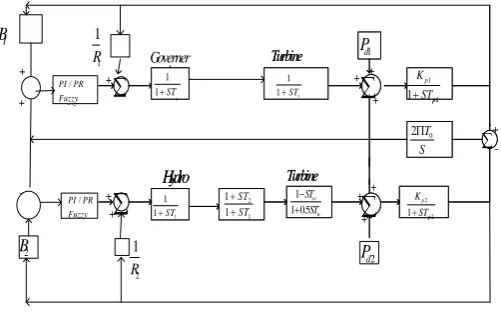
3. SYSTEM MODELING

The two-area interconnected power system taken as test system [4], In this study consists of thermal unit as area-1and hydro unit as area-2. The control task is to minimize the system frequency deviation



f

1

in area 1,

2

f



in area 2 and the deviation in the tie-line power flow



Ptie between the two areas under the load disturbances



Pd1 and



Pd2 in the two areas. This is achieved conventionally with the help of integral control which acts on

ACE

_iGiven by (1), which is an input signal to the controller where

ACE

_i the Area control error of the ith area

, 1 n

i tie ij i i

j

ACE

P

B f









 

₍₁₎



fi is Frequency error of ith area



Ptie, i j are Tie-line power flow error between ith and jth area

Bi is Frequency bias coefficient of ith area

1 1STg

1 1STt

1 1 1ST

2 1 1 1 ST ST   1 1 0.5 w w ST ST   Turbine Turbine Hydro / PI PR Fuzzy / PI PR Fuzzy 1 1 1 p p K ST  2 2 1 p p K ST  0 2 T S  1 d P     _       









_   1

1STg

1 1STt

1 1 1ST

2 1 1 1 ST ST   1 1 0.5 w w ST ST   Turbine Turbine Hydro /

P I P R F u z z y

/ PI PR Fuzzy 1 1 1 p p K ST  2 2 1 p p K ST  0 2 T S  2 d P    _       









_   / PI PR Fuzzy / PI PR Fuzzy Governer I B 2 B 1 1 R 2 1

R d2

P

1

d P

Fig (2)

The Above figure show the interconnection of Basic Two Power System, The Area Control Error of Each Unit is fed to Different controller and Response is Observed

.

4. DIFFERENT CONTROLLER

4.1 INTERGRAL CONTROLLER:

The conventional integral controller is implemented and objective of any controller of load frequency is to produce a controlling signal which keeps the frequency of given system constant and power exchange between control areas at predetermined values.Fig.1shows the typical scheme of conventional control on ith control area. The area control error(ACEi) is input to the PI controller with proportional gain (kp) [5]



i

K



i ACE Control Area 1 d P  di f  tie p  i

B

  i

u

Fig (3) shows the conventional controller

1

B

,

B

₂Are Frequency Bias Factors.

1 d

p



is Change in Load In Area 1

12

T

is the Tie Line Constant depends Upon the System Voltage of Two Control Area Connected Through the Tie line and Its Reactance

.

4.2 PID CONTROLLER

[image:2.595.55.269.134.286.2] [image:2.595.311.556.310.429.2] [image:2.595.38.289.574.731.2]

© 2017, IRJET | Impact Factor value: 5.181 | ISO 9001:2008 Certified Journal | Page 495

P

K

i

K

d

K

PLANT











 

U t

Figure (4)

( )

i

C S P d

K

G

K

K s

s







where kp, ki, kd are the proponational, integral and derivative Gains and above equation Can Be written in equivalent form of the PID Controllers

_{( )S p}

(1

1

_d

)

i

G

K

T s

T s







Where

T

_i



K

_p

/

K andT

_{i d}



K

_d

/

K

_p,

T andT

i d are

Known as Integral and Derivative Time Constants Respectively These controllers are used mostly in industrial application because of simple implementation, more reliable and easy realization. These controllers highly depend on tuning parameters. This problem can be removed by most popular Ziegler-Nichols method.

THE ZIEGLER-NICHOLS RULES (FREQUENCY RESPONSE METHOD)

TABLE-1

Controller

p

K

T

i

T

i

P 0.5ku

PI 0.4ku

_{/ 2}

u

T

PID 0.6ku

_{/ 2}

u

T

T

_u

/ 8

Each Area Transfer Function is Given by

 





















1

1

1

1

( )

2 2

1

1

g t

l

g t

s

T s

T s

s

s

p s

s

D

T s

T s

K

R













_

_

_

_

_

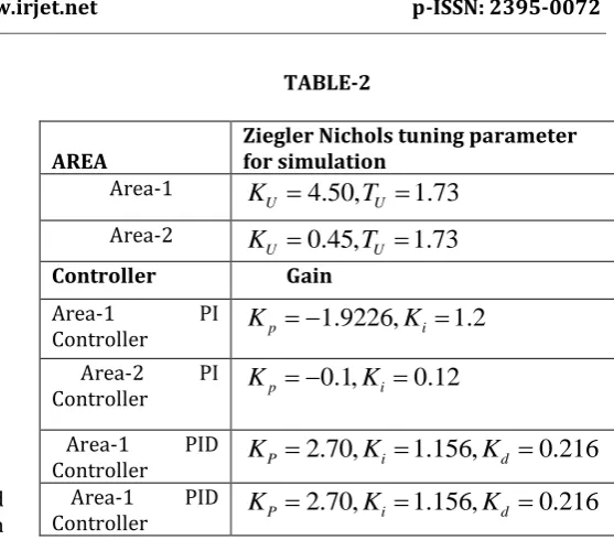
TABLE-2

AREA Ziegler Nichols tuning parameter for simulation

Area-1

_4.50,

_1.73

U U

K



T



Area-2

_0.45,

_1.73

U U

K



T



Controller Gain

Area-1 PI

Controller

K

p

 

1.9226,

K

i



1.2

Area-2 PI

Controller

K

p

 

0.1,

K

i



0.12

Area-1 PID

Controller

K

P



2.70,

K

i



1.156,

K

d



0.216

Area-1 PID

Controller

K

P



2.70,

K

i



1.156,

K

d



0.216

Simulation is Done for Two – Area system for 0.01pu load Change in Area-1 And Results Are Studied.

5. FUZZY LOGIC CONTROLLER

Fuzzy set theory and fuzzy logic establish the rules of a nonlinear mapping. There has been extensive use of fuzzy logic in control applications. Due to Non- Linearity of the System Parameters, PI and PID controllers with fixed gain parameters may not be provide better controlling of frequency deviation in multi area power system. This problem Can be solved by Using Fuzzy logic, Because the Output of a controller is Self Tunned Depend upon the Error. Fuzzy logic controllers are especially used for control those systems that are very typical to analyze by conventional controller means they are not well defined by mathematical formulation. One of its main advantages is that controller parameters can be changed very quickly depending on the system dynamics. [6]

The basic steps in modelling fuzzy based

controller after deciding the type of inference system

are:



Fuzzyfication of crisp values

1.Extraction and normalization of crisp values for input fuzzy vectors and output fuzzy vectors.

2. Selection of the membership functions (MFs)- number and shape, for input fuzzy vectors and output fuzzy vectors.

[image:3.595.285.564.68.313.2] [image:3.595.48.271.93.275.2]

© 2017, IRJET | Impact Factor value: 5.181 | ISO 9001:2008 Certified Journal | Page 496



Rule base and Fuzzy Inference

1. Form a rule base using control observations. 2. Find out the rule bases that are stored

3. The rule base consists of easy to form simple if-then conditional statements that decide the control objectives and control policy of the domain experts

.



Defuzzification

1. Calculate the crisp values for corresponding fuzzy output vector, applying a suitable defuzzification process.

2. Results are procured after simulation.

[image:4.595.313.552.252.698.2]

For the proposed controller, the Mamdani fuzzy inference engine was selected and realized by five triangular membership functions for each of the three linguistic variables (ACEi, d/dt(ACEi), Ki) with suitable choice of intervals of the membership functions where ACEi and d/dt(ACEi) act as the inputs of the controller and Ki is the output of the controller. NB, NS, Z, PS, PB represent negative big, negative small, zero, positive small, and positive big respectively. [8]

TABLE 3

ACE

NB NS Z PS PB





d

ACE

dt

NB PB PB PB PS Z

NS PB PB PB Z Z

Z PS PS Z NS NS

PS Z Z NS NB NB

PB Z NS NB NB NB

The suitable choice of intervals of the Memberships Functions was made as-0.1 to 0.1 for ACEi, -0.03 to 0.03 for d/dt(ACEi)); and 0.001 to 1 for Ki

System performance in respect of deviations ⧍f1, ⧍f2 and



Ptie for 0.01 p.u.MW step load change in area-1, using Fuzzy Controller is studied [9].

6. PROPONATIONAL CONTROLLER

The Basic structure of proponational Controller is Shown in Fig. (5)

( )

PR

K s

PLANT

( )

US







Figure (5)

The PR current controller

K

PR is represented by:

K

_PR

 

s

K

_p

K

_{i 2}

s

₂

s









where,

K

p is the Proportional Gain term,

K

i is the Integral

Gain term and



₀is the resonant frequency. The ideal resonant term on its own in the PR controller provides an infinite gain at the ac frequency



₀ and no phase shift and gain at the other frequencies

. [10]

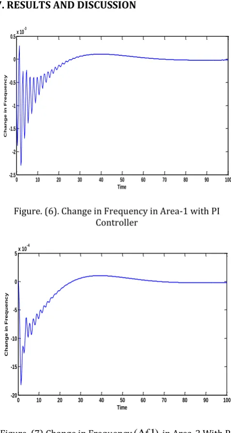
7. RESULTS AND DISCUSSION

0 10 20 30 40 50 60 70 80 90 100 -2.5

-2 -1.5 -1 -0.5 0 0.5x 10

-3

Time

C

h

a

n

g

e

i

n

F

r

e

q

u

e

n

c

y

Figure. (6). Change in Frequency in Area-1 with PI Controller

0 10 20 30 40 50 60 70 80 90 100 -20

-15 -10 -5 0 5x 10

-4

Time

C

h

a

n

g

e

i

n

F

r

e

q

u

e

n

c

y

[image:4.595.315.552.280.452.2] [image:4.595.30.282.413.511.2]

© 2017, IRJET | Impact Factor value: 5.181 | ISO 9001:2008 Certified Journal | Page 497

0 10 20 30 40 50 60 70 80 90 100 -4

-3 -2 -1 0 1 2x 10

-4

Time

C

h

a

n

g

e

i

n

F

r

e

q

u

e

n

c

y

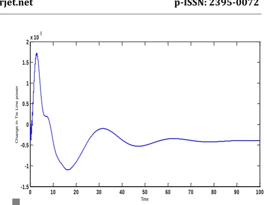
Figure. (8) Change in Tie-Power with PI Controller

0 10 20 30 40 50 60 70 80 90 100 -2.5

-2 -1.5 -1 -0.5 0 0.5 1 1.5

2x 10

-4

Time

C

h

a

n

g

e

i

n

F

r

e

q

u

e

n

c

y

Figure. (9) Change in frequency

(



f

1)

in Area-1 With PR Controller

0 10 20 30 40 50 60 70 80 90 100

-9 -8 -7 -6 -5 -4 -3 -2 -1 0 1x 10

Time

C

h

a

n

g

e

in

Fr

e

q

u

e

n

c

y

Figure. (10) Change in frequency

(



f

1)

in Area-2 with PR Controller

0 10 20 30 40 50 60 70 80 90 100

-1.5 -1 -0.5 0 0.5 1 1.5

2x 10

Time

C

h

a

n

g

e

i

n

Ti

e

L

in

e

p

o

w

e

r

Figure. (11) Change in Tie Line Power with PR controller

0 20 40 60 80 100 120 140 160 180 200

-5 -4 -3 -2 -1 0 1x 10

-3

Time

C

h

a

n

g

e

i

n

f

r

e

q

u

e

n

c

y

Figure. (12) Change in frequency

(



f

1)

in Area-1 With PID controller

0 50 100 150 200 250 300 -5

-4 -3 -2 -1 0 1x 10

-3

Time

C

h

a

n

g

e

i

n

F

r

e

q

u

e

n

c

y

[image:5.595.52.400.63.287.2] [image:5.595.296.566.69.276.2] [image:5.595.42.542.82.729.2] [image:5.595.312.549.316.490.2]

© 2017, IRJET | Impact Factor value: 5.181 | ISO 9001:2008 Certified Journal | Page 498

0 50 100 150 200 250

-10 -8 -6 -4 -2 0 2 4x 10

-4

Time

C

h

a

n

g

e

i

n

F

re

q

u

e

n

c

y

Figure. (14) Change in Tie-line power with PID controller

0 10 20 30 40 50 60 70 80 90 100 -5

-4 -3 -2 -1 0 1 2 3 4 5x 10

Time

C

h

a

n

g

e

i

n

Fr

e

q

u

e

n

c

y

Figure. (15) Change in Frequency in Area -1 With Fuzzy Logic

0 10 20 30 40 50 60 70 80 90 100 -5

-4 -3 -2 -1 0 1 2 3 4 5x 10

Time

C

h

a

n

g

e

i

n

Fr

e

q

u

e

n

c

y

Figure. (16) Change in Frequency in Area-2 With Fuzzy logic

0 10 20 30 40 50 60 70 80 90 100 -5

-4 -3 -2 -1 0 1 2x 10

C

h

a

n

g

e

i

n

Fr

e

q

u

e

n

c

y

Time

Figure. (17) Change in Tie-Line Power with Fuzzy Logic

0 10 20 30 40 50 60 70 80 90 100 -5

-4 -3 -2 -1 0 1 2x 10

Time

C

h

a

n

g

e

in

Fr

e

q

u

e

n

c

y

Fuzzy PI PR

Figure. (18) Change in frequency with different controllers

8. CONCLUSIONS:

From the above tabulated and plotted simulation results for the change in plant frequency and the tie line power, it is clear that the intelligent Fuzzy based control minimizes the settling time and maximum overshoot for change in system frequency (f) and tie- line power that is for 1% change in input power;1%change in frequency is observed Proponational resonant controller Gives Steady state error Minimum with Compromise of settling time. Thus the fuzzy control methodology is faster and accurate as compared to conventionally used PI, PID and PR controllers and Hence steady state is achieved faster in case of Fuzzy logic controllers for LFC of Two area system

9. APPENDIX

F=50 Hz, Ri=2.5 Hz/p.u. Megawatts, Tpi=20s, Tr=10s, Hi=5 s, Kr=0.499, Pri==2000-Megawatt, Tt-i=0.299s, Tgi=0.081s, Kpi=120 Hertz/p.u. Megawatts, Ki=4, Kd=5, Tw=1 s, Di=8. 331*10 -3 p.u Megawatt/ Hz, Bi=0.4254 p.u MegaWatt/Hz, ai=0.515, a= (2* pi*Ti ), del P di= 0.01, Kp=0.05,Ki=-0.01, Kd=0.01.

10. REFERENCES

[1] O. I. Elgerd, Electric Energy Systems Theory: An Introduction.

New York: McGraw-Hill, 1982.

[2] Nanda J, Kavi BL, “Automatic generation control of

interconnected power system,” IEE Proceedings, Generation, Transmission and Distribution, 1988; No. 125(5), pp.385– 390.

[3] Ibraheem, Prabhat Kumar and Kothari, D.P. (2005), “Recent Phlosophies of AGC Strategies in Power Systems”,

[image:6.595.39.281.66.223.2] [image:6.595.311.558.71.242.2] [image:6.595.43.280.260.394.2] [image:6.595.38.286.437.744.2]

© 2017, IRJET | Impact Factor value: 5.181 | ISO 9001:2008 Certified Journal | Page 499

[4] D. K. Chaturvedi, P. S. Satsangi, and P. K. Kalra, “Load

frequency control: A generalized neural network approach,” Elect. Power Energy Syst., vol. 21, no. 6, pp. 405–415, Aug. 1999

[5] Chang C.S., Fu W., “Area load-frequency control using fuzzy gain scheduling of PI controllers,” Electric Power System Research, Vol. 42, 1997, pp. 145-52.

[6] LEE, CC, “Fuzzy logic in control systems: Fuzzy logic controller Part-I&II,” IEEE Trans. Syst., Man, Cybern., vol. 20, no. 2, pp. 404-435, March-April 1992.

[7] Chang C.S., Fu W., “Area load-frequency control using fuzzy gain scheduling of PI controllers,” Electric Power System Research, Vol. 42, 1997, pp. 145-52

[8] Sathans S., Swarup A., “Intelligent load frequency control of two area interconnected power system and comparative analysis,” IEEE Xplore, International conference on communication systems and network technologies (CSNT 2011), pp. 360-365 E-ISBN 978-0-7695-4437-3.

[9]Sathans and A. Swarup, “Automatic Generation Control of Two-areaPower System with SMES: from Conventional to Modern and Intelligent Control,” International Journal of Engineering Science and Technology, vol. 3, no. 5, pp. 3693-3707, 2011.