Munich Personal RePEc Archive
Risk Aversion and the Value of Risk to
Life
Bommier, Antoine and Villeneuve, Bertrand
Risk Aversion and the Value of Risk to Life
Antoine Bommier
∗[email protected]
Bertrand Villeneuve
†[email protected]
June 10th, 2008
Abstract
The standard literature on the value of life relies on Yaari’s (1965) model, which
includes an implicit assumption of risk neutrality with respect to life duration. To
overpass this limitation, we extend the theory to a simple variety of nonadditively
separable preferences. The enlargement we propose is relevant for the evaluation of
life-saving programs: current practice, we estimate, puts too little weight on mortality
risk reduction of the young. Our correction exceeds in magnitude that introduced by
the switch from the notion of number of lives saved to the notion of years of life saved.
Keywords: Value of Statistical Life; Lifecycle Behavior; Cost-benefit Analysis.
JEL:D61, D81, D91, I18, J17.
1
Introduction
Billions of dollars are spent every year on mortality reduction programs. Issues like the
al-location of funds to medical research or prevention, the design of safety rules or the wording
of environmental bills raise intense debate on the relevance of the choices made by
govern-ments and their agencies. For economists, the baseline is that alternative projects should
∗Address: Toulouse School of Economics (CNRS, GREMAQ), 21 allée de Brienne, 31000 Toulouse, France.
†Address: CREST, Laboratoire de Finance Assurance, 15 boulevard Gabriel Péri, 92245 Malakoffcedex,
be evaluated with objective criteria to avoid pure waste or dramatic underinvestment in less
popular issues.
To back public decisions, some inquiry into individual valuation of life is indispensable.
In practice, if we leave apart contingent valuation, the analysis of the wage-risk tradeoffis
the major source of estimates of people’s behavior with respect to risk to life. These surveys
are primarily informative about industrial workers. Since public programs affect wider
pop-ulations whose characteristics may vary considerably and given that the mortality changes
considered are often beyond the range experienced by the reference sample, a theoretical
support for the interpretation of the data is indispensable.
The choice of the structural life-cycle model that minimizes bias at estimationand
extrap-olation stages is capital. The standard approach uses additively separable life-cycle models.
The intertemporal additivity assumption, which involves an implicit assumption of risk
neu-trality with respect to length of life (Bommier 2006) is extremely constraining. Although
this model has been severely criticized in other branches of literature, it remains an almost
universal assumption for applied economics on the value of life.1 Nearly all mortality-related
cost-benefit analyses rely, explicitly or not, on this assumption.
In this paper, we develop an alternative model, based on recursive von
Neumann-Morgen-stern utility functions, which relaxes the additivity assumption and thereby introduces what
we shall call mortality risk aversion. Although this extension complicates intermediate
calcu-lations, practical difficulties are kept at a reasonable level: formulas for the value of statistical
lives are almost as simple as those obtained with the standard additive model. There are
therefore no technical difficulties for applying this novel approach to concrete issues. Above
all, relaxing additivity warrants a significant gain in accuracy. As an illustration, we use
empirical results on the wage-risk tradeoff to calibrate both the additive and nonadditive
models. While the additive model proves unable to fit the data, the generalization proposed
provides an excellent fit with reasonable estimated parameters.
To emphasize the importance of accounting for mortality risk aversion, we compare the
benefits of (fictitious) life saving policies using different methods. The magnitude of the bias
caused by the additive separability assumption appears to be uncomfortably big. The type
of cost-benefit analysis that is currently recommended for life-saving programs is likely to be
strongly biased in favor of the elderly. The correction we suggest exceeds in magnitude that
introduced by the switch from the notion of number of lives saved to the notion of years of
life saved.
The structure of the paper is as follows. Section 2 positions our work in the recent
related literature. Section 3 recalls the additive model, introduces more general preferences
and characterizes mortality risk aversion. Section 4 shows the consequences of alternative
models for the individual valuation of statistical lives. Using an available hedonic regression
of the value of statistical life, Section 5 searches for the best fitting model and shows the
performance of the nonadditive version. Section 6 contrasts quantitatively several evaluation
procedures on typical life saving programs.
2
Related literature
Most of the economic literature on the Value of Statistical Life (henceforth VSL) is based
on a particular model whose standard version (e.g. Arthur 1981, Shepard and Zeckhauser
1984 or Rosen 1988) relies on elements developed in Yaari (1965). Several extensions have
recently been suggested.
In Murphy and Topel (2006),health multiplies the instantaneous utility derived from the
flow of consumption. Since health is assumed to be exogenous in that part of their paper
assessing the gain from mortality risk reduction, their approach is equivalent to assuming
that agents have additively separable utility functions whose (exogenous) discount function
is not necessarily exponential. Hall and Jones (2007) also extend Yaari’s model by
assuming in applications that it equals the inverse of the mortality rate. Though sensible,
this amounts to assuming that instantaneous utility depends on mortality through a
partic-ular functional form. Ehrlich and Yin (2005) model a technology through which protection
expenditures increase longevity; the authors also introduce a bequest motive.
The above contributions extended Yaari’s model in several directions, but have in common
that they all maintain the assumption of additive separability of preferences. It is precisely that later assumption that we shall relax. Our contribution is thus of a different nature:
instead of incorporating additional variables to Yaari’s model (such as health or bequest),
we explore the potential of a less straightly structured specification. As we shall see, this
provides different insights, especially on the speed at which VSL may or may not decline
with age at old ages.
The effect of age on the VSL is controversial.2 Simple simulations of the original models
exhibit either a decline with age, or an inverse U-shape. When careful calibration is achieved
to match empirical consumption profiles, the inverse U-shape is generally found, with a rather
slow decline at old ages. The above mentioned theoretical extensions of Murphy and Topel
(2006) and Ehrlich and Yin (2005) tend to confirm this prediction. Empirical works, however,
do not converge to a consensus on the relation between age and VSL. The hedonic regressions
on wages in Aldy and Viscusi (2003) and Kniesneret al. (2006) also show an inverse U-shape
relation between age and VSL, with a rather rapid decline of VSL at old ages. Other recent
works (Alberini et al. 2004, Smith et al. 2004, Aldy and Viscusi forthcoming), based either
on contingent valuation or wage-risk tradeoffs, tend to minimize the significant decline that
was apparent in previous estimates. The debate seems far from being closed. The present
paper contributes to it by showing that when the assumption of additive separability of
preferences is relaxed in order to account for mortality risk aversion, then a rapid decline of
VSL at old ages becomes theoretically plausible.
3
Lifetime preferences
3.1
Basic concepts and notation
We define a life as the cross product of an infinite consumption profile c and a finite age at
death T. For an individual of agea,a life(c, T)is an element of La with
La=C([a,+∞[,R)×[a,+∞[. (1)
where C([a,+∞[,R)denotes the set of continuous functions mapping [a,+∞[ into R. Con-sumption at age t is denoted by ct. Note that consumption is not a priori constrained to
equal zero for t > T, but this will have no importance since it will be assumed that agents do not care for consumption after death.
Lifetime being uncertain, modelling the tradeoff between mortality and consumption
requires a theory of choice under risk. We apply the VNM expected utility framework on
the space of lotteries (i.e. probability measures) over La. To do so, one can define a utility
function (or Bernoulli index) Ua(c, T) such that for any two probability measures η, η0 on
La,
ηºη0
⇔EηUa≥Eη0Ua, (2)
where º denotes weak preference and Eη (resp. Eη0) is the expectation operator based on
probability η (resp. η0).
We assume that individuals do not care for consumption after death, which amounts to
posing Ua(c, T) = Ua(c0, T) for any two c,c0 that are equal on [a, T]. This enables us to
normalize Ua so as to have Ua(c, a) = 0,∀c.
A probability measure overLa for which the consumption profilecis predetermined and
the uncertainty bears only on T can be written as δc×m where δc is a Dirac and m is a probability measure over [a,+∞) describing the distribution of the age of death. We have
Eδc×mUa = Z +∞
a
This expected utility will be simply denoted by EUa in the rest of the paper.
The probability of being alive at ageT, conditional on being alive at age a, is denoted
sTa ≡exp
µ −
Z T
a
µtdt
¶
= 1−
Z T
a
m(t)dt, (4)
where the latter equality expresses survival in terms of mortality rates, µt being the hazard rate of death at age t.
We make two purely technical assumptions.
Assumption 1 µt tends to infinity as t tends to infinity.
Assumption 2 cis bounded in the long run, i.e. there is an interval [cmin, cmax]withcmin >
0 and cmax<+∞ on which c is supported after some arbitrary date.
Integration by parts yields
EUa =
£ −sT
aUa(c, T)
¤+∞
a +
Z +∞
a
sT a
∂Ua(c, T)
∂T dT, (5)
and eventually, using Assumptions 1 and 2 (sT
a → 0 and Ua is bounded as T → +∞) to
evaluate the first term, we find
EUa =
Z +∞
a
sTa∂Ua(c, T)
∂T dT. (6)
The potential of the theory now depends on the assumptions that are made on Ua(c, T)
or equivalently on ∂Ua(∂Tc,T). We first come back on the common additive specification and
highlight some of its properties. Then we suggest a more general form forUa(c, T)on which
our analysis will be based.
3.2
The additive model
individual of age a has preferences represented by the Bernoulli index
Uadd
a (c, T) =
Z T
a
u(ct)e−λ(t−a)dt, (7)
where u is a well-behaved instantaneous utility function and λ is the subjective discount factor. In this case
∂Uadd
a (c, T)
∂T =u(cT)e
−λ(T−a), (8)
and the expected utility is
EUaadd =
Z +∞
a
sTau(cT)e−λ(T−a)dT. (9)
We recognize the formulation in Yaari (1965).
A peculiar feature of this model is that ∂Uaa d d(c,T)
∂T is independent of past consumption.
Said differently, the marginal utility of life is independent of how good (or bad) life has been
in the past.3 If we parallel this with wealth preferences, this is akin to assuming that marginal
utility of wealth is independent of wealth, i.e. that the decision maker is risk neutral. This
point wasfirst stressed by Broome (1993) who criticized the additive specification for relying
on an implicit assumption of “risk neutrality over discounted QALY’s”, which he qualified as
“surely implausible” (Broome, 1993, p.166). In a parallel line of argument, Bommier (2006)
shows that assuming additive separability as in (7) is equivalent to assuming risk neutrality
over life duration when considering consumption paths whose variations compensate for time
preferences.
3.3
The recursive model
One could think of several tractable options with marginal utility of life depending on past
consumption. The approach we follow preserves stationarity, one of the key properties of
Yaari’s specification.4 Basically, stationarity means that preferences are time consistent,
independent of age and of history (see Epstein 1983, who extended Koopmans’ 1965 definition of stationarity to the case of choice under uncertainty). In other words, people of different ages differ only with respect to their earning and mortality profiles. Bommier (2005) shows
in particular that for agents that are sure to die (but who may not know when they will die),
preferences are stationary if and only if they can be represented as
Ua(c, T) =
Z T
a
u(ct) exp
µ −
Z t
a
v(cτ)dτ
¶
dt. (10)
This specificationfirst appeared in the economic literature (in the case of immortal agents)
in Uzawa (1969). As soon as we depart from the additive case, the meanings of u and v
are not straightforward. Uzawa interpreted the integral Ratv(cτ)dτ as an “accumulated rate
of time preference”. This extrapolation from the additive model is misleading: it suggests
that the rate of time discounting depends on past consumption whereas, due to their
re-cursive form, preferences are indeed characterized by independence with respect to it.5 A
rigorous approach involves starting from well defined local properties of individual
prefer-ences (marginal rates of substitution) and deriving proper concepts of time discounting and
intertemporal elasticity of substitution, as will be done in Subsection 3.4.
Two special cases of the recursive model (10) must be highlighted at this stage. They
are equally simple and the empirical part of this paper will show a clear difference (in favor
of the second) in their abilities to fit data. The first one is simply the additive one (take
v(·) =λ, a constant). The second one is the multiplicative model in which v(c) =ku(c),∀c,
4Another possibility is to allow changes in risk aversion à la Kihlstrom and Mirman (1974). This is pursued in Bommier (2006). Instead of taking the expected value of Uadd
a (c, T), one uses Φ(Uaadd(c, T))
where Φis an increasing transformation. The drawback is that these preferences are not stationary, except in two cases: Φis linear (the additive case) orΦis exponential andλ= 0(the multiplicative model discussed later on in the present paper).
5To see recursivity, remark that for alla, b, T such thata≤b≤T
Ua(c, T) = Z b
a
u(ct) exp µ
−
Z t
a
v(cτ)dτ ¶
dt+ exp Ã
−
Z b
a
v(cτ)dτ !
for some constant k;equation (10) can be integrated to give
Uamulti(c, T) =
1−exp³−kRaT u(ct)dt
´
k . (11)
The term multiplicative refers to the fact that the exponentials of the instantaneous utilities
multiply each other. Being a concave transformation of an additive utility function, this
latter specification maintains the assumption of weak separability of preferences. Increasing
k amounts to increasing risk aversion in the sense of Kihlstrom and Mirman (1974). This specification is therefore particularly appropriate to illustrate the impact of risk aversion on
the value of risk to life.
Under uncertain lifetime, the expected utility based on (10) is
EUa =
Z +∞
a
stau(ct) exp
µ −
Z t
a
v(cτ)dτ
¶
dt. (12)
This paper will not discuss the consequences, for given mortality, of recursive preferences
on the intertemporal allocation of wealth.6 We focus instead on issues related to endogenous
mortality choices, a typical example of which being the wage-risk tradeoff. For this purpose,
we need a few general concepts.
3.4
Local properties
The first concept expresses how individuals trade offpresent and future consumptions:7
6Consumption smoothing with this kind of preferences is discussed at length in Bommier (2005) for nonconstant v. A causal link between mortality (as a risk) and apparent impatience is put forward. In particular, with the multiplicative model which rules out pure time preference, sizable impatience can be calculated even with small mortality rates.
7Because of our continuous time modelling, we use Volterra derivatives. They measure utility changes when consumption (or mortality) varies by an infinitesimal value during an infinitesimally short lapse of time. For example ∂Ua
∂µtdµdtgives the change inUawhen mortality rates increase bydµduringdtaroundt.
Definition 1 (RD) The mortality adjusted rate of time discounting at age t is
RD(c, t)≡ −d dtlog
µ
1
st a
· ∂EUa
∂ct
¶¯¯¯ ¯•
ct=0
. (13)
In absence of mortality at aget(i.e. if st
a were constant aroundt), RD(c, t)would be the
rate of time discounting in continuous time defined in Epstein (1987). The correction 1/sta
simply neutralizes the uncertainty effect that mortality risk has on consumption
(consump-tion is contingent on survival). With the recursive model, calcula(consump-tions yield
RD(c, t) = v(ct)u
0(c
t)−v0(ct)(u(ct)−µtEUt)
u0(c
t)−v0(ct)EUt
, (14)
where EUt is defined in (12). Although the definition of RD(c, t) is conditional on a, the
current age of the individual, RD(c, t) only depends on consumption and mortality at ages
greater than or equal to t. This is a consequence of history independence and time consis-tency: a 20 year old individual and a 50 year old individual anticipate the same value for
the rate of discount of consumption at age 60. The indexes defined below exhibit similar
properties of independence from the past.
The second concept, intertemporal elasticity of substitution, is defined with continuous
time as the limit of the direct elasticity of substitution (as defined in McFadden, 1963)
between consumptions at two different dates whose time distance tends to zero.
Definition 2 (IES) The intertemporal elasticity of substitution at age t, which we denote
σt, is defined by:
1
σt
δt≡lim τ→t τ6=t
−
∂2EUa (∂ct)2
∂EUa ∂ct
2 + 2
∂2EUa ∂ct∂cτ ∂EUa
∂ct ∂EUa∂cτ − ∂2EUa (∂cτ)2
(∂EUa
∂cτ )
2
1
ct∂EUa∂ct + 1
cτ∂EUa∂cτ
(15)
where δt is the Dirac delta function.8
The intertemporal elasticity of substitution, together with the mortality adjusted rate of
time discounting are the key determinants of the marginal trade-offs involved in consumption
smoothing. For example, in a perfect market environment (with actuarially fair annuities
and a rate of interest r), the growth rate of the optimal path would be(r−RD(c, t))σt.
With the recursive model,
σt =−
1
ct
u0(c
t)−v0(ct)EUt
u00(c
t)−v00(ct)EUt
. (16)
When preferences are additive or multiplicative, this formula simplifies to σt = −u 0(ct) ctu00(ct).
The third concept of time discounting simply expresses how people trade off survival probabilities at different ages.
Definition 3 (RDLY) The rate of time discounting for life years is defined by
RDLY(c, t)≡ −d dt log µ ∂EUa ∂st a ¶¯¯¯ ¯• ct=0 . (17)
With the recursive model,
RDLY(c, t) =v(ct). (18)
The fourth concept, which is at the center of our analysis, requires more comments and
clarifications.
Definition 4 (MRA) Mortality risk aversion is defined by
MRA(c, t)≡ lim
T→t T >t
∙ − d
dT log
µ
∂Ua(c, T)
∂ct
¶¸
. (19)
This coefficient is unaffected by an affine transformation of Ua, meaning that it
rep-resents a fundamental characteristic of individual preferences, independent of the specific
representation that was chosen. If the marginal utility of life extension is decreasing in past
The terminology “mortality risk aversion” emphasizes that MRA(c, t) corresponds to a
coefficient of risk aversion with respect to length duration along particular (and generally
not constant) consumption paths. Indeed, writing
∂Ua(c, T)
∂ct
= ∂Ua(c, T)
∂T ·
µ
∂Ua(c, T)
∂ct
Á
∂Ua(c, T)
∂T
¶
, (20)
one obtains
MRA(c, t)≡ −
∂2Ua(c,t)
∂t2
∂Ua(c,t)
∂t
+ lim
T→t T >t
d dT log
̶Ua(c,T)
∂T ∂Ua(c,T)
∂ct
!
. (21)
The first term in the RHS is recognizable as a coefficient of risk aversion with respect to life
duration. When consumption profiles such that
lim
T→t T >t
d dT
̶Ua(c,T)
∂T ∂Ua(c,T)
∂ct
!
= 0 (22)
are considered, MRA(c, t) and the Arrow-Pratt coefficient are equal.
Consumption profiles that comply with (22) are characterized by the fact that the
mar-ginal rate of substitution between additional life years and consumption just before death is
independent of the age at death. In particular, (22) amounts to having u(ct)e−λt constant
in the additive model, and ct is constant with the multiplicative model. In both cases, this
can be interpreted as having a constant flow of felicity (Bommier, 2006).
The decomposition into two terms is important for understanding the origin of MRA(c, t),
but quite remarkably, with the recursive model any consumption profile leads to the following
simple expression
MRA(c, t) = v
0(c t)u(ct)
u0(c t)
, (23)
which depends only on local properties. Remark that MRA(c, t)>(<)0if v(·) is increasing
4
The value of statistical lives
Subsection 4.1 defines the value of statistical lives (VSL) and relates this index with the
structural parameters of the recursive model. Subsection 4.2 shows the information one can
draw from empirical data to estimate preference parameters.
4.1
VSL
A natural concept to deal with choices involving mortality changes is the marginal rate of
substitution between mortality and consumption:
Definition 5 (VSL) The value of a statistical life at age t > a is defined by
VSL(c, t)≡ −
µ ∂EUa ∂µt ¶Á µ ∂EUa ∂ct ¶ . (24)
An agent of age t is ready to give up VSL(c, t)·dµ·dt in consumption to save dµ·dt
statistical lives. This is how we construe the term “Value of Statistical Life”, although it may
differ from other definitions that can be found in the economic literature.9 By derivation
from (12), one obtains
VSL(c, t) = EUt u0(c
t)−v0(ct)EUt
. (25)
The following expression relates VSL to survival probabilities and discount rates.
Proposition 1 For any consumption profile
VSL(c, t) =
Z +∞
t
sτt u(cτ) u0(c
τ) exp µ − Z τ t
ρ(c, τ0)dτ0
¶
dτ . (26)
with
ρ(c, τ0) =RD(c, τ0)−MRA(c, τ0) + 1 στ0
•
cτ0 cτ0
. (27)
Proof. See appendix.
In the additive case, withct=c(a constant), this expression simplifies to
VSL(c, t) = u(c) u0(c)
Z +∞
t
sτte−λ(τ−t)dτ . (28)
This formula has been known for years and its simplicity explains its success. It is considered
very convenient since, if we abstract from consumption variations, VSL is proportional to a
discounted sum of life years. The relation between age and VSL is then computable from
a standard life table and a discount rate. This way of accounting for age was initially
introduced by Moore and Viscusi (1988) and is now used and recommended by agencies
like the USA Environmental Protection Agency (EPA) and the Office of Management and
Budget (OMB) for cost-benefit analyses.
Proposition 1 is associated with a minor increase in complexity. Although the
general-ization makes intermediate calculations more fastidious, we eventually find that the benefit
of saving one statistical life among individuals of a given age is also proportional to the
dis-counted sum of years at risk. Casually, we find that accounting for consumption variations
is relatively simple, whether preferences are additive or not.
There are two notable differences between the additive and the recursive models. First, in
the recursive model the mortality adjusted rate of discount RD is not constant. Instead of
us-ing a discount functione−λ(τ−t), as in the additive case, we have to useexp¡−Rτ
t RD(c, τ 0)dτ0¢.
Actually, when we calibrate the model (Section 5), we find that the variations of RD remain
limited until advanced ages, so this first difference can be considered as minor. The second
difference is much more significant: years of life have to be discounted with the mortality
adjusted rate of discount (RD) minus mortality risk aversion (MRA).
Consequently, the greater mortality risk aversion, the faster VSL declines as a function of
age. This is fairly intuitive: a risk averse agent is willing to pay more to avoid the chance of a
major loss. In terms of mortality, a loss would be an early death. The additive model, which
4.2
Wage-risk tradeo
ff
The revealed preferences argument can be invoked to show how occupational choices provide
information about utility functions. Assume that, at all ages, an individual has to choose
between jobs that differ with respect to wage and instantaneous fatality risk. Let µ0
t be the
exogenous baseline mortality rate at age t. For an extra instantaneous mortality µt (total
mortality being µ0
t +µt), the wage is denoted by w(t, µt). Labor income can be used for
consumption or savings. We denote by k= (kt)t≥0 the age-specific saving profile defined by
kt≡w(t, µt)−ct. (29)
For our purpose, we do not need to fully specify the lifetime budget constraints that are
related to the intertemporal markets and their possible imperfections. We will simply assume
that these constraints (possibly infinitely many) only bear on the function k and that each
of them is Volterra differentiable. We denote the set of constraints byK.
We may think of different kinds of constraints. With non storable commodities and no
intertemporal markets, kt = 0 for all t. Another possibility would be a single constraint of
the form R0∞kthte−rtdt = 0 with r being the rate of interest and h = (ht)t≥0 an exogenous
function. This includes the important case of intertemporal markets, in particular life
annu-ities.10 We could also imagine that the constraints K have the form R0tkτe−rτdτ ≥ 0 for all
t. That would be the case in a world where there is no annuity market, no borrowing and a rate of return on savings equal to r. More complex market imperfections can be thought of. Undoubtedly, allowing any kind of constraints onkleaves us with a fairly high degree of
generality, although certain cases are not covered (e.g. nonlinear consumption taxes).
10To be more specific, exogenously priced life annuities are considered. Endogenous prices would mean that prices change as the consumer changes his mortality e.g. via activity choice. This case is not included here; ifhwere equal to the (endogenous) survival function, as with perfect intertemporal markets, the VSL
Using (4) and (12), we rewrite the lifetime utility function of an agent of agea as
EUa(c, µ) =
Z +∞
a
u(ct) exp
µ −
Z t
a
(µτ +µ0
τ +v(cτ))dτ
¶
dt. (30)
A rational agent solves the maximization program
max
µ,c EUa(
c, µ)s.t. K. (31)
Following the terminology of Aldy and Viscusi (2003, henceforth A&V), the derivative
wµ(t, µ) = ∂w∂µ(t,µ) is called the “wage-risk tradeoff.” Even without an explicit formulation of
the constraints K, we can show that at the optimal choice the wage risk tradeoff and the
VSL are equal. Indeed, differentiating (29), for all t, τ ,we have µ
∂
∂µt +wµ(t, µt) ∂ ∂ct
¶
kτ = 0. (32)
Letc∗ andµ∗ denote the optimal consumption and mortality paths. As we assumed that all
constraints can be written as functions of k, the first order conditions ensure that for all t,
utility cannot be improved without violating the constraints. Thus, because of (32), it must
be the case that at the optimum
µ
∂
∂µt +wµ(t, µt) ∂ ∂ct
¶
EUa= 0. (33)
Therefore:
wµ(t, µ∗t) =−
µ
∂EUa(c∗, µ∗)
∂µt
¶Á µ
∂EUa(c∗, µ∗)
∂ct
¶
=VSL(c∗, t). (34)
The observation of the wage-risk tradeoffreveals VSL and makes the calibration of the utility
function possible. Compared to similar results, the strength of the latter equation is that it
5
Data
fi
tting
5.1
Method
As explained in Viscusi and Aldy (2003), a hedonic regressionfits the envelope of the choices
made by the workers in the sample. Since the envelope is tangent to individual indifference
curves, the prediction based on the hedonic regression for a vector of individual characteristics
can be interpreted as the VSL for the corresponding worker. We base the calculations on
this fundamental observation.
As discussed in Section 2, several recent contributions estimated the relation between age
and VSL from hedonic regressions, providing contrasting results. As an illustration, we use
the result of one of them (A&V) to calibrate our model. By doing so, we do not claim to
provide undisputable estimates of the true preference parameters since they are conditional
on the particular empirical age—VSL relationship we employ. Nevertheless, we comply with
the objective of the paper: showing that relaxing additivity parsimoniously can significantly
improve the ability of the structural model to fit the data. The consequences for policy
recommendations are far from trivial.
We use the parameters given by A&V in their Table 4:
wµAV(t) =−1.92×10⁷ + 1.88×10⁶ t−4.54×10⁴ t2+ 335.24t3 (35)
where t ∈ [18,62], expresses the individual’s age in years, and wµ the yearly wage in 1996
Dollars. The calibration strategy we pursue involves searching the parameters of the recursive
model that best fit equation (35).11
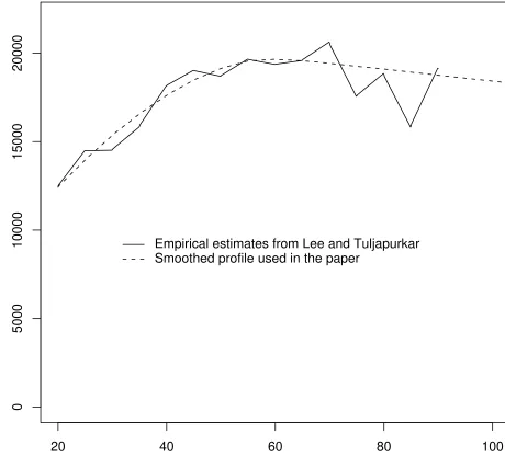
In order to calibrate the model, we also need the age-specific consumption profile c∗,
which is not available in the dataset used by A&V. The optimal consumption profile cannot
be deduced from the theoretical model without specification of the constraints K, on which
we have limited knowledge. Rather than posing specific constraints, we approximated c∗
with a smoothed version of the age specific individual consumption profile reported in Lee
and Tuljapurkar (1997) (see Figure 1 for the original estimates and the smoothed profile that
we use).12
5.2
Goodness of
fi
t
The first question that we may address is whether we can reproduce (35) with the standard
additive model (namely,v=λ=Constant andu(c) = c1−γ
1−γ−u0for some constantsu0 andγ).
The answer is positive, but with very implausible parameters. Indeed the distance minimizing
discount rate is−8.1%,which explains94%of the age-related variance in equation (35). Had we constrained the rate of discount to be greater than or equal to 3% (to approach values
that are considered as reasonable), we would have at best explained 58% of the age-related
variance.
At this point it is legitimate to wonder whether this poor fit is due to the fact that
we only considered isoelastic instantaneous utility functions, or more fundamentally to the
additive separability. We relax each of these assumptions in turn.
If we simply requireuto be increasing and concave rather than isoelastic, we can obviously improve the fit. By considering rates of discount greater than or equal to 3%, we can
now explain 79% of the age-related variance. The gain in explanatory power might seem
significant but, in fact, it is quite disappointing when we recall that we added an infinity of
degrees of freedom to the model (u is now nonparametric). This control stage adds weight to our view that structure (additive/nonadditive) matters much more that specification
(isoelastic/nonparametric), which we now illustrate.
In fact, keepinguisoelastic but in the recursive form appears to be a much more efficient way to improve the predictive power of the model. We explored the case where u(c) =
c1−γ
1−γ −u0 andv=λ+βu; compared to the standard additive model (β = 0), this structure
requires only one additional degree of freedom. Moreover it encompasses the multiplicative
age-model (obtained when λ = 0) described in Subsection 3.3, which has the same number of degrees of freedom as the standard additive model. In Figure 2, we report the minimum
distance (the sum of squares) between the theoretical predictions and the empirical estimates,
the survival weighted average RD being constrained to take particular values given on the
horizontal axis. The results obtained with the additive and the multiplicative models are
also reported. The distance on the vertical axis has been normalized so that the distance
between the empirical VSL and its mean equals 1.
Opting for the recursive model dramatically increases the capacity of the theory to
re-produce empirical VSL. Even if we constrain the mortality adjusted rate of discount to take
reasonable positive values we still obtain an excellent fit. We can constrain the
survival-weighted average RD to take any value between 3 and 7%, and still explain more than 95%
of age-related variability of the wage-risk tradeoff. This is much better than the additive
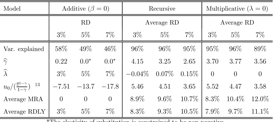
model which only explains from 42 to 58% thereof. Table 1 reports the model’s performance
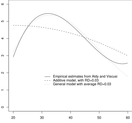
(variance explained and parameters) for a range of discount factors. Figure 3 illustrates the
fits obtained when the average mortality adjusted rate of discount is constrained to equal
3% in both models. Interestingly enough, one can see from Table 1 or Figure 2 that when
RD is constrained to plausible positive values, the multiplicative model does a much better
job than the additive one, with the same number of degrees of freedom. Therefore even if
Model Additive (β= 0) Recursive Multiplicative (λ= 0)
RD Average RD Average RD
3% 5% 7% 3% 5% 7% 3% 5% 7%
Var. explained 58% 49% 46% 96% 96% 95% 95% 96% 89%
b
γ 0.22 0.0∗ 0.0∗ 4.15 3.25 2.65 3.70 3.77 3.56
b
λ 3% 5% 7% −0.04% 0.07% 0.15% 0 0 0
u0/(c 1−γ
1−γ) 13 −7.51 −13.7 −17.8 5.46 4.51 3.65 5.52 4.47 3.58
Average MRA 0 0 0 8.9% 9.6% 10.7% 8.3% 10.4% 12.0%
Average RDLY 3% 5% 7% 8.3% 9.3% 10.5% 7.9% 9.7% 11.1%
[image:21.595.75.545.89.300.2]*The elasticity of substitution is constrained to be non-negative.
Table 1: Calibration and performance.
5.3
Evaluated parameters
For the recursive model, as apparent in Figure 2, the curve representing the distance between
predicted and actual values exhibits a flat shape around the minimum; in practice this
means that the combination of parameters that optimally fit the data is difficult to state.
The observation of the relation between age and VSL may not suffice to calibrate all the
parameters of the model with precision.
This is not surprising given the theoretical results provided in Section 4. From equation
(26) we know that what matters for determining the variations of wµ along the life cycle
is mainly the combination of two elements: the mortality adjusted rate of discount (RD)
minus mortality risk aversion (MRA). If consumption were constant along the life cycle, we
would expect empirical observation of VSL to be informative about the difference between
RD and MRA, and not about each of them separately. Though in our case consumption is
not constant, which in principle should solve the identification problem, our estimates suffer
from the same kind of indeterminacy. For each value of RD we find the best value of MRA,
Ultimately, to discriminate more sharply between the several likely possibilities, we should
integrate data on behavior patterns that go beyond the wage-risk tradeoff. One possibility
would be to look at consumption smoothing behavior (in order to estimate RD from
an-other source), but we leave that aside for lack of adequate data. Results thereafter are
systematically reported for RD taking values 3, 5 and 7%.
5.4
Practical consequences
From the last two rows of Table 1, it is possible to get afirst idea about the bias generated by
the additive assumption. While the additive model constrains mortality risk aversion to be
absent, the recursive model gives estimates that range from 8.9% to 10.7%. In other words,
when people discount consumption with rates of 3, 5 and 7%, life years in VSL should be
discounted with rates of −5.9%, −4.6% or −3.7% respectively. The additive model, which imposes the same rate of discount for consumption as for life years, is likely to cause a huge
bias.
Should that lead to a major shift in policy recommendations? The next section shows
that RDLY gives the rate of discount to be used for estimating the welfare equivalent of a
statistical life. While the additive model constrains RDLY to equal the rate of discount, the
more general model shows values of RDLY that exceed those of RD by several percentage
points. This means that the additive model puts too much relative weight on the elderly.
We see now how large the bias can be in practice.
6
Welfare evaluation
6.1
Objective
In order to evaluate the social benefits of mortality risk reductions, a well defined social
objective is required. The utilitarian approach axiomatized by Blackorbyet al(1997) involves
at birth. The social welfare function is then given by
X
i
e−λSbiUi
0, (36)
where the sum is taken over all individuals,λS is the social discount rate, bi is the birth year
of individual i andUi
0 is his expected utility at birth.
We use Arthur’s (1981) terminology. The welfare equivalent of a statistical life for
indi-vidual i is defined by
WE(c, t)≡ −∂U
i
0
∂µt, (37)
where candµare individuali’s consumption and mortality. WE has a fairly simple
expres-sion in the general case:14
WE(c, t) =
Z +∞
t
sτ0u(cτ) exp
µ −
Z τ
0
RDLY(c, τ0)dτ0
¶
dτ . (38)
Like the VSL, the welfare equivalent is a discounted sum of life years. With the additive
model RDLY=RD,thus it is correct to use the discount rate inferred from empirical studies on consumption smoothing to estimate the welfare equivalent of a statistical life. With the
recursive model, RDLY is typically greater than the rate of time preferences estimated in
studies on consumption smoothing. Thus, omission of mortality risk aversion generates a
pro-old age bias in the welfare evaluation of mortality risk reduction.
6.2
Methods
We describe now thefive evaluation methods for a program that we will apply in the following
subsection.
14From (4), it follows that
∂sτ a
∂µt = 0ifτ < t, and ∂sτ
a ∂µt =−s
τ
aifτ≥t.
Method 1: The number of lives saved. Though there is no economic support for this
method, it has been frequently used in the past. EPA and OMB still recommend reporting
the number of lives saved.
Method 2: Utilitarianism with the additive utility function. The benefit of a
pro-gram is measured by the social welfare function (36). Individuals are assumed to have the
same additive utility function, with a rate of time preference of 3, 5 and 7%, the other
parameters being drawn from Section 5. The social rate of discount is taken equal to the
individual rate of time preference.
Method 2’: Aggregate WTP with additive utility function. Assumptions on
indi-viduals are the same as for method 2. The benefit of a program is now evaluated by the sum
of the individuals’ willingness to pay for such a program.
Method 3: Utilitarianism with the recursive utility function. Similar to method
2, with the recursive model as estimated in Section 5. The average survival weighted RD
and the social rate of discount are constrained to 3, 5 and 7%.
Method 3’: Aggregate WTP with the recursive utility function. Similar to method
2’, with the recursive model as estimated in Section 5. The average survival weighted RD
and the social rate of discount are constrained to 3, 5 and 7%.
In principle, method 2’ (respectively 3’) amounts to method 2 (respectively 3) only if one
presumes that the marginal social value of consumption is equal across people of different
ages; in other words, if redistribution is perfect. In practice, since the distribution of wealth is
far from ideal with respect to the social welfare function, it has been argued that aggregate
willingness to pay cannot be considered as a relevant policy indicator. The issue is not
specific to life saving programs but general to any cost benefit analysis (see for example
the discussion in Blackorby and Donaldson 1990). In the case of mortality reduction, Pratt
aggregating individual willingness to pay may actually be a particularly misleading indicator.
Despite these shortcomings, method 2’ remains the most commonly employed in the applied
literature.
6.3
Application
To show the magnitude of distortion in the evaluation of safety programs, we consider two
fictitious programs that are assumed to have the same cost. One that decreases mortality
rates proportionally and another that decreases mortality rates uniformly. For example, we
could think of air quality alerts15 on the one hand and of earthquake surveillance on the
other.
We denote these hypothetical interventions as A and B. Policy A is characterized by a
proportional reduction of mortality rates
µt→(1−εA)µt, (39)
and policy B by a uniform reduction of mortality rates
µt→µt−εB. (40)
whereεA andεB are positive constants. We take the age structure of the population and the
baseline mortality rates observed in the USA in 1999. We also assume that A saves twice
as many (statistical) lives as B. Policy A is mostly effective for older people (and babies)
while policy B saves lives uniformly. Figure 4 shows the age distribution of lives saved (it
has been scaled so that A saves 2000 statistical lives while B saves only 1000). We assume
that the consumption profile is c∗ (see Subsection 5.1), for ages above 20. For ages below
20, and especially for babies and children, the assumption that preferences are independent
of age becomes problematic. The low levels of consumption that are typically observed
in the very first years of life would then imply very high marginal utility of consumption,
and therefore very low values of statistical lives. This is hard to buy. To circumvent this difficulty, we maintain the assumption that preferences are independent of age and assume
that consumption is the same between birth and 20. Of course this option is arbitrary, one of its merits being that most of the difference between A and B is based on effects on the
adults, for which estimates are more reliable.
Intuitively, it is not very clear whether A or B should be preferred. On the one hand A
saves more lives. On the other hand B saves younger people, who still have many years of
life before them. We use the above five types of benefit evaluation.
The results are summarized in Table 2. By assumption, A is twice as efficient as B from
the viewpoint of method 1. The additive model in methods 2 and 2’ provides an age-adjusted
value of a statistical life, so the conclusion is different. Methods 2 and 2’ predict that the
benefits of A and B are of about the same size. The fact that B saves less lives than A is
approximately compensated by the fact that it saves younger people. The question now is
whether this age adjustment and this conclusion are correct. Methods 3 and 3’ suggest that
they are not. With the recursive model, the benefits of B appear to be much greater than
those of A. The correction related to the introduction of mortality risk aversion is anything
but negligible. Passing from the additive model to the nonadditive one is a bigger step than
passing from the traditional method (number of lives saved) to the additive model.16
Discount rate
Method for benefit evaluation 3% 5% 7%
1. Number of lives saved 0.5 0.5 0.5
2. Utilitarianism with additive utility 1.11 0.97 0.88
3. Utilitarianism with recursive utility 3.23 2.64 2.18
2’. Aggregate WTP with additive utility 0.94 0.82 0.75
3’. Aggregate WTP with recursive utility 1.95 1.75 1.72
Table 2: Benefits of B/Benefits of A.
EPA guidelines advise performing sensitivity analysis by calculating the results of both
methods 1 and 2’. As the results of method 2’ are known to depend on the rate of discount,
about which there is no general agreement, they advise reporting the results for different
rates lying in the 3—7 % interval, in order to provide a reasonable confidence interval.
Unfor-tunately, the additive model is so restrictive that the truth may be way outside this interval.
The methods currently used by EPA and OMB (and indirectly by policymakers) are likely
to be significantly distorted in favor of the old.
7
Conclusion
Most economists would agree that predicting saving behavior under the assumption of risk
neutrality would make little sense. They would also vehemently criticize a fund manager
who decides to “optimize” investment under the assumption that members are risk neutral.
However, the economic literature on the value of a statistical life has endorsed a similar
choice. It focused on a specification that paid little attention to the fact that mortality
makes our life akin to an extraordinary lottery. Is it reasonable to assume that individuals
are risk neutral with respect to length of life? And to evaluate life saving programs under
this assumption?
These questions have been addressed in this paper. On the theoretical side, the story is
clear. Mortality risk aversion makes individual willingness to pay for mortality risk reduction
decline more rapidly with age. Although intermediate calculations are sometimes fastidious,
we eventually found that accounting for mortality risk aversion is fairly simple. Just like with
the standard additive model, estimating VSL and welfare benefits associated to mortality risk
reduction simply involves computing weighted sums of life-years saved. The rates of discount
to be used must however account for both time preferences and mortality risk aversion.
tions, about 40 years have passed and a number of empirical studies tried to measure risk
aversion with respect to lotteries on wealth. No consensus has emerged. There is no reason
to believe that preferences with respect to lotteries on the length of life will be easier to
as-sess. It would be excessively optimistic to expect that a single study could provide a robust
estimate of mortality risk aversion. This should be rather seen as a long term objective that
will probably require the collection of specific data.
However, in order to clarify the ideas at stake, we used results from a recent empirical
study on the relation between VSL and age to estimate plausible values of mortality risk
aversion. The theoretical extension neatly improved the quality of fit. We found that this
index of risk aversion is likely to be positive and greater than the rate of time discounting.
In other words, accounting for mortality risk aversion may even be more important than
accounting for time preferences.
The contrast between ourfindings and the dominant economic approach is striking. While
the notion of time preferences has been pointed out as being a critical element to estimate
the value of a statistical life, the standard method simply rules out mortality risk aversion.
It seems that “the paradigm of optimizing a simple functional form” (to take Rubinstein’s
2003 words) has led economists to ignore a key ingredient of individual preferences. The
consequence is that cost-benefit analysis produced for the allocation of public money across
life saving programs is likely to be strongly distorted.
References
[1] Alberini, A., M. Cropper, A. Krupnick, and N. Simon, 2004, “Does the Value of a Statistical
Life Vary with Age and Health Status? Evidence from the U.S. and Canada.” Journal of
Environmental Economics and Management, 48(1): 769-792.
[2] Aldy, J.E. and W.K. Viscusi, 2003, Age Variations in Workers’ Value of Statistical Life. NBER
[3] Aldy, J.E. and W.K. Viscusi, forthcoming, “Adjusting the Value of a Statistical Life for Age
and Cohort Effects.” Review of Economics and Statistics.
[4] Arrow, K.J., 1971, Essays in the Theory of Risk Bearing. Chicago: Markham.
[5] Arthur, W.B., 1981, “The Economics of Risks to Life.” American Economic Review, 71(1):
54-64.
[6] Blackorby, C., W. Bossert and D. Donaldson, 1997, “Birth-Date Dependent Population Ethics:
Critical-Level Principles.” Journal of Economic Theory, 77(2): 260-284.
[7] Blackorby, C. and D. Donaldson, 1990, “A Review Article: The Case against the Use of the
Sum of Compensating Variations in Cost-Benefit Analysis.” Canadian Journal of Economics,
23(3): 471-494.
[8] Bommier, A., 2006, “Uncertain Lifetime and Inter-temporal Choice: Risk Aversion as a
Ra-tionale for Time Discounting.” International Economic Review, 47(4): 1223-1246.
[9] Bommier, A., 2005, Life Cycle Theory for Human Beings. Working Paper, University of
Toulouse.
[10] Broome, J., 1993, “Qalys.” Journal of Public Economics,50(2): 149-176.
[11] Browning, M., 1991, “A Simple Nonadditive Preference Structure for Models of Household
Behavior over Time.” Journal of Political Economy, 99(3): 607-637.
[12] Carrasco, R., J. Labeaga and J. López-Salido, 2005, “Consumption and Habits: Evidence
from Panel Data.” Economic Journal, 115(500): 144-165.
[13] Deaton, A., 1974, “A Reconsideration of the Empirical Implications of Additive Preferences.”
Economic Journal, 84(334): 338-348.
[15] Epstein, L.G., 1983, “Stationary Cardinal Utility and Optimal Growth Under Uncertainty.”
Journal of Economic Theory, 31: 133-52.
[16] Epstein, L.G., 1987, “A Simple Dynamic General Equilibrium Model.” Journal of Economic
Theory, 41: 68-95.
[17] Epstein, L.G. and S.E. Zin, 1991, “Substitution, Risk Aversion, and the Temporal Behavior
of Consumption and Asset Returns: An Empirical Analysis.” Journal of Political Economy,
99(2): 263-286.
[18] Ehrlich, I. and Y. Yin, 2005, “Explaining Diversities in Age-Specific Life Expectancies and
Values of Life Saving: A Numerical Analysis.” Journal of Risk and Uncertainty, 31(2): 129-162.
[19] Hall, R.E. and C.I. Jones, 2007, “The Value of Life and the Rise in Health Spending.” Quarterly
Journal of Economics, 122(1): 39-72.
[20] Hayashi, F., 1985, “The Effect of Liquidity Constraints on Consumption: A Cross-Sectional
Analysis.” Quarterly Journal of Economics, 100(1): 183-206.
[21] Johansson, P.O., 2002, “On the Definition and Age-Dependency of the Value of a Statistical
Life.” Journal of Risk and Uncertainty, 25(3): 251-263.
[22] Kihlstrom, R.E. and L.J. Mirman, 1974,.“Risk Aversion with Many Commodities.” Journal
of Economic Theory, 8(3): 361-88.
[23] Kniesner, T.J., W.K. Viscusi, and J.P. Ziliak, 2006, “Life-Cycle Consumption and the
Age-Adjusted Value of Life.” Contributions to Economic Analysis & Policy: 5(1):Article 4.
[24] Lee, R.D. and S. Tuljapurkar, 1997, “Economic Consequences of Aging for Populations and
Individuals Death and Taxes: Longer Life, Consumption, and Social Security.” Demography,
34(1): 67-81.
[25] McFadden, D., 1963, “Constant Elasticity of Substitution Production Functions.” Review of
[26] Moore, M.J. and W.K. Viscusi, 1988, “The Quantity Adjusted Value of Life.” Economic
Inquiry, 26: 368-388.
[27] Muellbauer, J., 1988, “Habits, Rationality and Myopia in the Life-cycle Consumption
Func-tion.” Annales d’Economie et de Statistique, 9: 47-70.
[28] Murphy, K.M. and R.H. Topel, 2006, “The Value of Health and Longevity.” Journal of Political
Economy, 114(5): 871-904.
[29] Pope, C.A. 3rd, M.J. Thun, M.M. Namboodiri, D.W. Dockery, J.S. Evans, F.E. Speizer and
C.W. Jr Heath, 1995, “Particulate Air Pollution as a Predictor of Mortality in a Prospective
Study of U.S. Adults.” American Journal of Respiratory and Critical Care Medicine, 151(3
Pt 1): 669-74.
[30] Pratt, J., 1964, “Risk Aversion in the Small and in the Large.” Econometrica, 32: 122-136.
[31] Pratt, J.W. and R.J. Zeckhauser, 1996, “Willingness to Pay and the Distribution of Risk and
Wealth.” Journal of Political Economy, 104(4): 747-763.
[32] Richard, S.F., 1975, “Multivariate Risk Aversion, Utility Independence and Separable Utility
Functions.” Management Science, 22(1): 12-21.
[33] Rosen, S., 1988, “The Value of Changes in Life Expectancy.” Journal of Risk and Uncertainty,
1: 285-304.
[34] Rubinstein, A., 2003, “ ‘Economics and Psychology’ ? The Case of Hyperbolic Discounting.”
International Economic Review, 44: 1207-1216.
[35] Ryder, H.E. Jr. and G.M. Heal, 1973, “Optimum Growth with Intertemporally Dependent
Preferences.” Review of Economic Studies, 40(1): 1-33.
[36] Shepard, D.S. and R.J. Zeckhauser, 1984, “Survival versus Consumption.” Management
[37] Smith, V.K., M.F. Evans, H. Kim, and D.H. Taylor, 2004, “Do the Near-Elderly Value
Mor-tality Risks Differently?” Review of Economics and Statistics, 86(1): 423-429.
[38] Uzawa, H., 1969, “Time Preference and the Penrose Effect in a Two-Class Model of Economic
Growth.” Journal of Political Economy, 77(4): 628-652.
[39] Viscusi, W.K. and J.E. Aldy, 2003, “The Value of a Statistical Life: A Critical Review of
Market Estimates throughout the World.” Journal of Risk and Uncertainty, 27(1): 5-76.
[40] Yaari, M.E., 1965, “Uncertain Lifetime, Life Insurance, and the Theory of the Consumer?”
Review of Economic Studies, 32(2): 137-150.
A
Proof of Proposition 1
In the proof, VSL stands for VSL(c, t) and RD for RD(c, t).We start from (25) and we use
the fact that
dEUt
dt = (µt+v(ct))EUt−u(ct) (41)
to compute
d
dtlogVSL= (42)
µt+v(ct)−
u(ct)
EUt −
u00(c
t)−v00(ct)EUt
u0(c
t)−v0(ct)EUt •
ct+v0(ct)
(µt+v(ct))EUt−u(ct)
u0(c
t)−v0(ct)EUt
.
Using (14) and (16), we get
d
dtlogVSL=µt+
1
σt •
ct
ct
+RD− u(ct)
EUt
. (43)
From (25), we obtain
EUt =
u0(c t)VSL
1 +v0(c t)VSL
thus
u(ct)
EUt
= u(ct)(1 +v
0(c
t)VSL)
u0(c t)VSL
= u(ct)v
0(c t)
u0(c t)
+ u(ct)
u0(c t)
1
VSL. (45)
Combining (45) with (43) yields
d
dtlogVSL=µt+
1
σt •
ct
ct
+RD− u(ct)v
0(c t)
u0(c t) −
u(ct)
u0(c t)
1
VSL, (46)
i.e.
dVSL
dt =
Ã
µt+RD− u(ct)v
0(c t)
u0(c t) + 1 σt • ct ct !
VSL− u(ct)
u0(c t)
. (47)
We show now in three steps that
VSL(c, t) =
Z +∞
t
sτt u(cτ) u0(c
τ) exp µ − Z τ t
ρ(c, τ0)dτ0
¶
dτ (48)
with
ρ(c, τ0) =RD(c, τ0)− u(cτ)v
0(c τ)
u0(c τ) + 1 στ • cτ cτ . (49)
Step 1. It is easy to see that the RHS of (48), if it converges, is a solution to the ODE
(47).
Step 2. Remark thatEUt >0. Indeed, a natural assumption is that the marginal value of
life years, which is proportional to u, is positive, and u >0 impliesEUt >0.
Given Assumptions 1 and 2,EUttends to zero ast tends to infinity. This and (25) imply
that VSL→ 0 as t → +∞. We can also conclude from this, (14) and EUt > 0, that RD is
bounded below in the long run. Consequently, ρ(c, t)→+∞ ast→+∞. This implies that
the RHS of (48)→ 0 as t → +∞. VSL and the RHS of (48) have therefore the same limit when t→+∞.
Step 3. The ODE (47) being linear, if we denote byythe difference between the VSL and
Given that ρ(c, t)→+∞ ast →+∞, y goes to infinity when t→+∞if it’s not null. This
0
5000
10000
15000
20000
US Dollars Empirical estimates from Lee and Tuljapurkar
[image:35.517.22.482.57.485.2]Smoothed profile used in the paper
Distance between theoretical predictions and A&V
−0.15 −0.10 −0.05 0.00 0.05 0.10 0.15
0.0
0.1
0.2
0.3
0.4
0.5
0.6
0.7
0.8
●
● General model
[image:36.517.43.482.52.464.2]Additive model Multiplicative model
0
1
2
3
4
5
6
Million dollars
Empirical estimates from Aldy and Viscusi Additive model, with RD=0.03
[image:37.517.29.486.59.483.2]Number of statistical lives saved (per one year age class)
[image:38.517.37.484.64.459.2]Intervention A Intervention B
Figure 4: Distribution of lives saved
0 10 20 30 40 50 60 70 80 90 100 110
0
5
10
15
20
25
30
35
40
45
50
55