http://dx.doi.org/10.4236/ojapps.2014.44016
How to cite this paper: Taniguchi, M. (2014) The Impact of Liberalization on the Production of Electricity in Japan: Stochas-tic Frontier Analysis. Open Journal of Applied Sciences, 4, 155-167. http://dx.doi.org/10.4236/ojapps.2014.44016
The Impact of Liberalization on the
Production of Electricity in Japan: Stochastic
Frontier Analysis
*
Miyuki Taniguchi
Graduate School of Economics, Keio University, Tokyo, Japan Email: miyuki@z3.keio.jp
Received 30 January 2014; revised 5 March 2014; accepted 12 March 2014
Copyright © 2014 by author and Scientific Research Publishing Inc.
This work is licensed under the Creative Commons Attribution International License (CC BY). http://creativecommons.org/licenses/by/4.0/
Abstract
This study aims to measure the impact of liberalization on the efficiency of electricity production in Japan using Stochastic Frontier Analysis (SFA). In addition, this study also aims to examine whether or not economies of scale exist in the electricity generation sector and the transmission sector, and whether or not economies of scope exist between electricity generation and transmis-sion. Since 1995, liberalization of the electricity market in Japan has been phased in and regula-tions on entry have been relaxed three times. One motivation for these regularity changes has been to improve the efficiency of electricity production by introducing competition. Using a panel data set on the nine main power companies in Japan over the period 1970-2010, estimates of fixed-effects and stochastic frontier models of the cost function are obtained and compared. Esti-mates of the cost function show that liberalization has improved cost efficiency when both frontier models and non-frontier models are estimated. Estimates of the fixed-effects model are used to calculate economies of scale and economies scope because the data support the fixed-effects mod-el. Economies of scope are found to exist for all nine power companies, while overall economies of scope declined in the 1970s and have improved little by little since the 1980s.
Keywords
Cost Function; Electricity; Liberalization; Stochastic Frontier Analysis; Economies of Scope; Vertical Integration
1. Introduction
Recently inefficiencies in the Japanese electricity market have been the focus of some attention. In particular, even though the liberalization of the electricity market has been phased in and regulations on entry have been relaxed three times since the 1990s, the monopolistic nature of the Japanese electricity market has been the
subject of much discussion since the Management and Coordination Agency in Japan (Soumu-cho) proposed
enegry liberalization (the official website of Federation of Electric Power Companies of Japan:
http://www.fepc.or.jp/enterprise/jiyuuka/keii/). There has also been some discussion of the possible separation of electricity generation and transmission. For example, Goto and Inoue (2012) measure the economies of scope between generation and transmission in Japan to examine the effectiveness of diversification in the Japanese
electricity industry [3]. This study aims to measure the impact of recent liberalizations on the efficiency of
elec-tricity production in Japan, and to examine whether or not economies of scope exist between elecelec-tricity genera-tion and transmission.
A huge literature has examined whether or not inefficiencies exist in various industries including the electric-ity industry. Papers using a parametric approach tend to estimate a cost function rather than a production tion because there are endogeneity problems associated with input choices when estimating a production func-tion. To estimate either a production function or a cost function, papers in the literature use either a parametric approach or a non-parametric approach. Papers using a non-parametric approach typically employ Data Enve-lopment Analysis (DEA) to measure the inefficiencies among the electricity companies. Papers using DEA measure either productive efficiencies or cost efficiencies, using the variables which are the same as the va-riables to estimate either the production function or cost function.
For the electricity industry in Japan, there are three key papers using parametric approach. Using data from 1978 to 1998, Kuwabara and Ida (2000) estimate a translog cost function for the Japanese electric companies
together with share equations [4]. Kuwabara and Ida (2000) aim to measure the extent of economies of scale and
economies of scope in the electricity industry in Japan, but they do not examine the impact of the liberalization measures that have been implemented. Their results support the existence of both overall economies of scale and economies of scope for all electric power companies during the period Kuwabara and Ida analyzed. Using data from 1982 to 1997, Nemoto and Goto (2006) estimate a constant elasticity of substitution (CES) cost function,
and measure the technical and allocative efficiencies of the transmission-distribution of electricity in Japan [5].
Their results show the existence of technical and allocative inefficiency. The observed costs are estimated to be from 9% to 48% higher than their efficient levels. Kinugasa (2012) measures the Lerner index for each Japanese electric company to examine whether three liberalizations have made the market more competitive using
esti-mates of translog production functions [6]. Kinugasa’s (2012) empirical results show that the three liberali-
za-tions have made every electricity market more competitive. Goto and Inoue (2012) estimate a composite cost
function for the Japanese electric companies using data between 1990 and 2008 [3]. Goto and Inoue do not use
the translog cost function, but rather use a composite cost function which enables them to measure the econo-mies of vertical integration, which includes both the effects of econoecono-mies of scale and econoecono-mies of scope, in electricity production. They reports that there were no overall economies of scale and that there were economies of scope. In detail, the economies of scale for generation existed during their sample period, while economies scale for transmission did not exist.
For the electricity industry in Japan, there are two key papers using the DEA approach. Tsutsui (2000) meas-ures the inefficiencies of Japanese electric companies using the Malmquist Index, and then compares the esti-mated inefficiencies of Japanese electric power companies with those of the US companies between 1992 and
2000 [7]. Although his results show that Japanese firms are more efficient than US firms, Tsutsui does not
ex-amine the impact of the electricity liberalization. One disadvantage of the DEA approach is that the statistical significance of the input variables cannot be evaluated. Hence, the impact of any liberalization cannot be ex-amined via the DEA statistically. Hattori, Jamasb, and Pollitt (2005) measure the efficiencies of electricity dis-tribution in the UK and Japan between 1985 and 1998, using not only stochastic frontier analysis (SFA), but also
DEA [8]. Their results show that the Japanese electricity system is less efficient than the UK system. Their data
period contains only the first electricity liberalization in Japan though Japan experienced three electricity libera-lizations in total up to now.
contri-bution of this study is to examine the impact of the liberalization in the Japanese electricity market by estimating a translog cost function directly. The second contribution of this paper is to measure the economies of scale and the economies of scope, using estimates of this translog cost function. As a result, the hypothesis that the three electricity liberalizations contribute to reducing the cost of electricity generation and transmission is supported.
This result is consisted with Kinugasa (2011) [6]. The estimates of the overall economies of scale and the
economies of scope in this paper are consisted with the results in Goto and Inoue (2012) [3]. The estimated
re-sults of this paper suggest that overall economies of scale did not exist and economies of scope existed.
The rest of this paper is organized as follows. Section 2 provides an outline of the key liberalizations of the electricity market that have been implemented in Japan. Section 3 discusses the empirical models that are used to examine the impact of these liberalizations and how this model can be used to check for the existence of economies of scope between electricity generation and electricity transmission, while Section 4 details the defi-nitions of the variables used and the data sources. Estimation results are reported in Section 5, and Section 6 contains a conclusion.
2. Liberalization of the Electricity Market
[image:3.595.92.536.518.709.2]In the 1990s, deregulation to reduce inefficiencies in the electricity market was popular all over the world. At that time, many European countries and the United States deregulated their electricity markets. Since 1995, li-beralization of the electricity market in Japan has been phased in and the regulations on entry have been relaxed three times. This liberalization aimed to improve the structural efficiency of firms in the industry and to reduce electricity bills that were said to be higher than the average level paid by consumers in foreign countries (Ya-maguchi (2007) [9]).
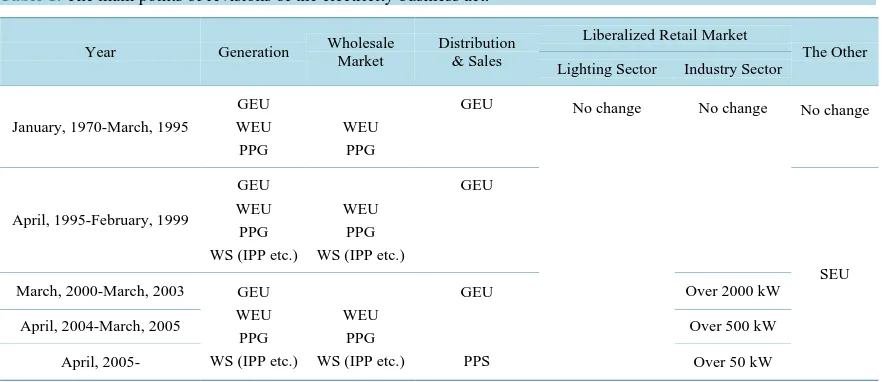
Table 1summarises the details of the main changes in the electricity market as a result of the liberalizations.
Prior to 1995, Japan was divided into ten geographic regions, and within each region a monopoly on power
gen-eration and distribution was allocated to one general electric power utility (GEU, Ippan Denkijigyousha). As a
result, there are ten general electric power utilities in Japan [9]. These ten companies each engaged in the
gener-ation, transmission and distribution of electricity within their respective geographical regions. Apart from GEUs,
only wholesale electric power utilities (WEU, Oroshiuri Denkijigyousha) were allowed to generate electric
power that was then supplied to GEUs. Only two WEUs existed; the Electric Power Development Company
Limited (Dengenkaihatsu) and the Japan Atomic Power Company (Nihon Genshiryokuhatsuden). Both
compa-nies were started with capital from the GEUs. Private power generation (PPG) was also allowed. In other words, the electricity generation was allowed as long as they sell the electric power to the others. After the collapse of Japan’s overheated stock and real estate markets in the early 1990s, higher electricity bills in Japan compared to those paid by consumers in foreign countries became an issue. The Japanese government aimed to improve the efficiency of electricity production by introducing competition into the electric power market.
Table 1.The main points of revisions of the electricity business act.
Year Generation Wholesale Market
Distribution & Sales
Liberalized Retail Market
The Other Lighting Sector Industry Sector
January, 1970-March, 1995
GEU WEU PPG
WEU PPG
GEU No change No change No change
April, 1995-February, 1999
GEU WEU PPG WS (IPP etc.)
WEU PPG WS (IPP etc.)
GEU
SEU March, 2000-March, 2003 GEU
WEU PPG WS (IPP etc.)
WEU PPG WS (IPP etc.)
GEU
PPS
Over 2000 kW
April, 2004-March, 2005 Over 500 kW
April, 2005- Over 50 kW
First, the Electricity Business Act (Denkijigyouhou) was revised to enable wholesale suppliers (WS) to enter the wholesale markets for electricity supply. This revision was enacted in December 1995. The typical example
of a WS is an independent power producer (IPP, Dokuritsukei Hatsudenjigyousha). IPPs include not only the
subsidiaries of GEUs but also companies like steel companies which have the knowhow to generate electric powers. In this context, the wholesale market for electricity refers to the generation of electricity in Japan. The electricity generated by the new entrants was sold to the general power companies, and then supplied to consumers through the transmission sectors owned and operated by the general electricity utilities. Since the
first revision of the Electricity Business Act, the specified electricity utilities (SEU, Tokutei Denkijigyousha),
who have a duty to generate, distribute, and sell electricity only for the specified areas, have started to generate and distribute electricity. However, the area served by a SEU has been an independent market.
In March 2000, the Electricity Business Act was revised again so that power producer and suppliers (PPS,
Tokuteikibo Denkijigyousha) could enter the retail markets for electricity, that is, PPS could sell electricity directly to consumers. This revision permitted new entry of suppliers into the retail market for electricity for consumers with an electric power contract of over 2000 kW. The remaining part of the retail market, that is, for small contract consumers, was maintained as a monopoly of the relevant regional electric power company. That is why this second revsion is called a partial liberalization.
In 2003, the Electricity Business Act was revised to allow entry in April 2004 into the retail market where each consumer’s electric power contract was over 500 kW, and then where each consumer’s electric power con-tract was over 50 kW in April 2005. In short, this revision expanded the sections of the retail market where the PPSs could enter. That is why this is called an expansion of the partial liberalization. Moreover, the market rules
for the electricity transmission sector and a watchdog organization (Souhaidengyoutou Gyomushienkikan) have
been established to realize fair deals.
An examination of how the retail market shares of various operators have changed after the electricity liber-alization began shows that the maximum market share of the PPSs was 0.74% after the PPS entered the retail
market ([10], p. 32). The ten main electric power companies have been able to maintain a market share of 70% -
80% even after the electricity liberalization ([10], p. 32). However, as a result of new entry, electricity prices
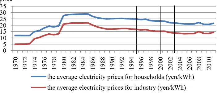
[image:4.595.123.474.521.673.2]have fallen. After the electricity liberalization began, average prices have tended to decline. This fact suggests that the existence of innovation by competition might have led to lower prices.
Figure 1 shows declines in the average electricity prices for households and industry around the time of the
liberalizations. After the first electricity liberalization, the average electricity prices for households and industry
tend to decline. Though Figure 1 suggests that all of three liberalizations seemed to be effective, there is a
pos-sibility that innovation in electric power generation affects electricity prices. Therefore, in the next section, the impacts of these three-step-liberalizations on the production of electricity are examined, using an econometric model.
Figure 1.Average electricity prices. Source: constructed by the author using data from the “Elec-tricity Statistics Information (Denryoku Toukeijouhou)” published by the Federation of Electric Power Companies of Japan. Notes: the three vertical lines show the years when the three electric-ity liberalizations were enacted.
0 5 10 15 20 25 30 35
1970 1972 1974 1976 1978 1980 1982 1984 1986 1988 1990 1992 1994 1996 1998 2000 2002 2004 2006 2008 2010
the average electricity prices for households (yen/kWh)
3. Model
3.1. Translog Frontier Cost Function
Assume that in the generation, transmission and distribution of electricity there are three inputs, labor, capital and fuel, and two outputs, the generation of electricity, and the transmission and distribution of electricity. These inputs and outputs are assumed to be related by a translog cost function. The number of inputs and the number
of outputs are defined following Goto and Inoue (2012) [3]. The outputs are measured as the total quantity
elec-tric power sold in a fiscal year and the total length of transmission routes, respectively. This assumption makes it easier to estimate the economies of scope between the generation and transmission & distribution sectors. To measure the inefficiency due to technical factors, a stochastic frontier version of the translog cost function is employed. Once the symmetry of the second derivatives of the cost function with respect to two different input prices is taken into account, the stochastic frontier translog cost function can be written as follows:
(
)
(
)
(
)
(
)
(
)
2 2
0 1 1 2 2 1 1 2 2 3 3 11 1 22 2
2 2 2
12 1 2 11 1 22 2 33 3 12 1 2
23 2 3 31 3 1 11 1 1 1
1
ln ln ln ln ln ln ln ln
2
1 1 1
ln ln ln ln ln ln ln
2 2 2
ln ln ln ln ln ln
it it it it it it it it
it it it it it it it
it it it it it it
TC y y p p p y y
y y p p p p p
p p p p y p
α α α β β β γ γ
γ δ δ δ δ
δ δ ρ ρ
= + + + + + + +
+ + + + +
+ + + + 2 1 2 13 1 3
21 2 1 22 2 2 23 2 3 1 1 2 2 3 3
ln ln ln ln
ln ln ln ln ln ln ln
it it it it
it it it it it it t t t
thermal it nuclear it new it it it
y p y p y p y p y p D D D t thermal nuclear new u v
ρ
ρ ρ ρ τ τ τ
ϕ ϕ ϕ
+
+ + + + + + +
+ + + + +
(1)
( )
lnTCit = f ⋅ +uit+vit, (2)
where TCit is the total cost of the i-th firm at time t, yjit is the quantity of the j-th output for the i-th firm at
time t, pkit is the observed price of the k-th input for the i-th firm at time t, Dst is a 0 - 1 dummy variable
taking the value of 1 if at time t the s-th change of the electricity liberalization has been implemented (s = 1, 2,
3) and zero otherwise, t is a time trend, thermalit is the ratio of thermal power generation to hydroelectric
generation for the i-th firm at time t, nuclearit is the ratio of nuclear power generation to hydroelectric
generation for the i-th firm at time t, newit is the ratio of new energy generation to hydroelectric generation
for the i-th firm at time t, αj, βk, γjl, δkm, ρjk, τs, ϕthermal, ϕnuclear, and ϕnew are coefficients to be
es-timated,uit is the inefficiency term for the i-th firm at time t, and vit is a standard disturbance. In this model,
it is assumed that all firms have the same production technology.
3.2. Method for Estimating Economies of Scale
When a 2 output cost function is assumed, the economies of scale for yit is defined as
ln ln
it it oit it
oit
it oit it oit
MC TC y TC s
AC y TC y
∂ ∂
= = ⋅ =
∂ ∂ (3)
where soit is the economies of scale for the o-th output, MCit is marginal cost, and ACit is average cost.
Equation (3) means that there are economies of scale when average cost is larger than marginal cost. Therefore,
when soit is larger than 1, there are no economies of scale. When soit is less than 1, there are economies of
scale.
In the case of this paper, the economies of scale for y1it and y2it are defined as
1it 1 11ln 1it 12ln 2it 11ln 1it 12ln 2it 13ln 3it
s =α γ+ y +γ y +ρ p +ρ p +ρ p (4)
2it 2 22ln 1it 12ln 1it 21ln 1it 22ln 2it 23ln 3it
s =α +γ y +γ y +ρ p +ρ p +ρ p (5)
In the case of two outputs, the overall economies of scale are measured as follows:
1 2 1 1 ln ln ln ln it it it it
it it it it it it
it it
it it it it
TC TC
y y
MC y y MC y y
SCL MC
AC TC TC TC
∂ + ∂
∂ ∂
= = ⋅ = = (6)
are economies of scale. Combining (3) and (6), the overall economies of scale can be defined as
1it 1it 2it 2it it
it
y s y s SCL
TC
+
= (7)
3.3. Method for Estimating Economies of Scope
Baumol, Panzar and Willing (1982) [11] define economies of scope as being complementary if
2
1 2
0
it
it it
TC y y
∂ <
∂ ∂ . (8)
One interpretation of Equation (8) is that for costs to be complementary the marginal cost of each output will decline when the amount of the other output increases. The second derivative on the left hand side of Equation (8) can be computed using (1) as:
[
]
2
12 1 2
1 2 1 2 1 2 1 2 1 2
ln ln ln
ln ln ln ln
it it it it it it
it it
it it it it it it it it it it
TC TC TC TC TC TC
s s
y y y y y y y y y y γ
∂ ∂ ∂ ∂
= + ⋅ = + ⋅
∂ ∂ ∂ ∂ ∂ ∂ . (9)
In Equation (9), 12
1 2 TC
y y
is always positive because TC12, y1, and y2 are all positive. Therefore, to see if
(9) is satisfied, it is only necessary to examine the sign of the following expression:
12 12 1 2
it it it
SCP =γ +s ⋅s (10)
Since this is a function of unknown parameters and the values of the explanatory variables, it needs to be evaluated using estimates of the paramters and the sample values of the explanatory variables.
3.4. Estimated Model
Equation (1) with uit =0 gives rise to a simple pooling model was given. Since the data being used to estimate
the cost function are panel data,it is natural to estimate Equation (1) allowing for inidvidual firm effects that are
either fixed and random effects. In this case, uit is a time-invariant random variable that is correlated with the
explanatory variables for the fixed effects model. In addition to these standard panel models, some stochastic frontier models are estimated in this study to allow for possible existence of stochastic inefficiencies. To try and capture any cost inefficiencies, four models are assumed: the pooling Stochastic Frontier (SF) model; the random-effects SF model; the fixed-effects SF model; and the Battese and Coelli (1992) Time Varying
Stochastic Frontier (TV-SF) model [12]. The estimated models are as follows;
Pooling Stochastic Frontier Model
( )
(
2)
(
2)
lnTCit = f ⋅ +uit+vit, uit ~HN 0,σµ ,vit ~N 0,σv , (11)
Tine Invariant SF Model
( )
(
2)
(
2)
lnTCit = f ⋅ + +ui vit, ui ~HN 0,σµ ,vit ~N 0,σv , (12)
Fixed-Effects SF Model
( )
(
2)
(
2)
lnTCit = f ⋅ +ζi + +ui vit, ui ~HN 0,σµ ,vit ~N 0,σv , (13)
Battese and Coelli Time Varying SF Model
( )
{
(
)
}
(
2)
(
2)
lnTCit = f ⋅ +uit+vit, uit =exp −η t−Ti u ui, i~HN 0,σµ ,vit ~N 0,σv , (14)
where ui, and uit are measures of technical inefficiency, vit is standard disturbance, ζi is the individual
fixed effect, Ti is the number of observations on firm i in the panel data set, N and HN denote a nornal
Equation (12) can be obtained as a special case of Equation (13) by imposing the restriction ζ =i 0 for all i,
and as a special case of Equation (14) by imposing the restriction η=0. The pooling model can be obtained as
a special case of Equations (11) and (12) by imposing the restriction σ =µ2 0. If σ =µ2 0 in all these models,
then the pooling model is chosen. The standard fixed effects models is nested within Equation (13) and can be
obtained by imposing σ =µ2 0. The standard random effects model and any one of the stochastic frontier models
are non-nested models.
4. Data
Data on the corporate accounts of the ten general electricity utilities are drawn from the “Electricity Statistics
Information (Denryoku Toukeijouhou)” published by the Federation of Electric Power Companies of Japan.
Though ten general electricitiy utilities have existed in Japan since 1970, Okinawa Electric Power Company is
excluded from the analysis in this study. The reason for this is that electricity production by Okinawa Electric
has some important characteristics that differ from other companies. For example, the scale of electricity
production at Okinawa Electric is much smaller than at the other companies. In addition, Okinawa Electric is the
only general electricity utility not using nuclear energy for electric power generation. Finally, the prefecture of
Okinawa is made up of a number of small islands where Okinawa Electric is obliged to generate and supply
electricity. As a result, it is thought that Okinawa Electric Power Company has a unique production function and
a unique cost function. Hence, a balanced panel data set consisting of annual data on the other nine general electricitiy utilities from 1970 to 2010 is used.
12
TC is total costs measured in million yen. The output in the electricity generation sector, y1it, is defined as
the total quantity of electric power sold to consumers in the lighting and power sectors (MWh). The output in
the transmission sector, y2it, is defined as the length in kilometers of the transmission route including both
overhead and underground routes. The unit fuel cost, p1it (million yen), is defined as
(
)
(
)
1
total fuel expenses . total quantity of fuel inputs
it it
it
p = (15)
The gross fixed capital is employed for the cost of capital, p2it (million yen). It is defined as
(
)
2it it it 1 t
p = DE GFC− +LPR , (16)
1 1 1 1
it it it it
GFC − =EUFA− +FAP− +IA− (17)
where p2it is the cost of capital for the i-th firm in year t, 𝐷𝐷𝐷𝐷𝑖𝑖𝑖𝑖 is the depreciation expenses for the i-th firm
in year t, GFCit−1 is the gross fixed capital for the i-th firm in year t−1, 𝐿𝐿𝐿𝐿𝐿𝐿𝑖𝑖 is the long-term prime rate
for loans made by the main Japanese banks in year t, EUFAit−1 is the fixed assets for the i-th firm in year 1
t− , FAPit−1 is the fixed assets in process for the i-th firm in year t−1, and IAit−1 is investment and other
assets for the i-th firm in year t−1. Data on the long-term prime rate for loans made by the main Japanese
banks are drawn from the “Bank of Japan Statistics” published by Bank of Japan. The personal expenses per worker per year, p3it(million yen), is defined as
(
)
(
)
3
personal expenses
the number of workers
it it
it
p = . (18)
1
D is a 0 - 1 dummy variable taking the value of 1 in 1995-2010, D2 is a 0 - 1 dummy variable taking the
value of 1 in 2001-2010, and D3 is a 0 - 1 dummy variable taking the value of 1 in 2004-2010. These three
dummy variables correspond to the three entry related liberalizations discussed in Section 2.
Table 2 provides desciptive statistics on all the relevant variables. The variables LNC, LNY1, LNY2, LNP1,
LNP2, and LNP3 in Table 2 refer to the natural logs of TCit, y1it, y2it, p1it, p2it, p3it, respectively. The
va-riable LNT in Table 2 refers to the natural log of the year. The variables THERMAL, NUCLEAR, and NEW in
Table 2 are the ratio of the quantities of electricity generation of thermal power, nuclear power, and new energy
to hydraulic power, respectively.
5. Results and Discussion
Table 2. Descriptive statistics.
Variable Mean Std. Dev. Minimum Maximum
LNC 13.588 0.992 10.874 15.682
LNY1 17.684 0.847 15.817 19.511
LNY2 8.977 0.594 7.829 9.957
LNP1 −3.734 0.546 −5.256 −2.685
LNP2 1.543 0.631 0.472 2.299
LNP3 2.041 0.505 0.676 2.751
D1 0.390 0.488 0 1
D2 0.244 0.430 0 1
D3 0.171 0.377 0 1
LNT 7.596 0.006 7.586 7.606
THERMAL 5.699 3.159 0.537 17.145
NUCLEAR 2.639 2.791 0.000 12.955
[image:8.595.133.465.302.710.2]NEW 0.026 0.083 0.000 0.462
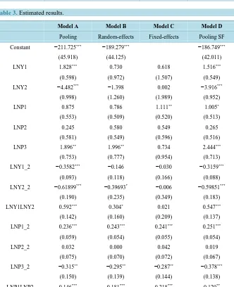
Table 3. Estimated results.
Model A Model B Model C Model D
Pooling Random-effects Fixed-effects Pooling SF Constant −211.725*** −189.279*** −186.749*** (45.918) (44.125) (42.011) LNY1 1.828*** 0.730 0.618 1.516***
(0.598) (0.972) (1.507) (0.549) LNY2 −4.482*** −1.398 0.002 −3.916*** (0.998) (1.260) (1.989) (0.952) LNP1 0.875 0.786 1.111** 1.005*
(0.553) (0.509) (0.520) (0.513)
LNP2 0.245 0.580 0.549 0.265
(0.581) (0.549) (0.596) (0.516) LNP3 1.896** 1.996** 0.734 2.444*** (0.753) (0.777) (0.954) (0.713) LNY1_2 −0.3582*** −0.146 −0.030 −0.3159***
(0.093) (0.118) (0.166) (0.088) LNY2_2 −0.61899*** −0.39693* −0.006 −0.59851***
(0.190) (0.235) (0.349) (0.183) LNY1LNY2 0.592*** 0.304* 0.021 0.547*** (0.142) (0.160) (0.209) (0.137) LNP1_2 0.236*** 0.243*** 0.241*** 0.251*** (0.059) (0.054) (0.055) (0.054)
LNP2_2 0.032 0.000 0.042 0.019
Continued
(0.055) (0.051) (0.053) (0.052) LNP2LNP3 0.264*** 0.281*** 0.391*** 0.218**
(0.092) (0.087) (0.092) (0.086)
LNP1LNP3 0.054 0.069 0.062 0.067
(0.064) (0.059) (0.060) (0.060) LNY1LNP1 −0.015 −0.029 −0.067** −0.026 (0.030) (0.027) (0.029) (0.028) LNY1LNP2 −0.098*** −0.078** −0.036 −0.100*** (0.036) (0.036) (0.043) (0.031) LNY1LNP3 0.018 −0.008 0.025 −0.006 (0.048) (0.052) (0.066) (0.043) LNY2LNP1 0.017 0.048 0.079** 0.030
(0.037) (0.034) (0.035) (0.035) LNY2LNP2 0.165*** 0.104** 0.004 0.172*** (0.052) (0.050) (0.059) (0.047) LNY2LNP3 −0.162** −0.119* −0.063 −0.142** (0.065) (0.063) (0.072) (0.060)
D1 −0.070*** −0.066*** −0.058** −0.072*** (0.026) (0.024) (0.024) (0.027)
D2 −0.153*** −0.141*** −0.151*** −0.150*** (0.025) (0.023) (0.023) (0.023)
D3 −0.157*** −0.127*** −0.120*** −0.154*** (0.028) (0.026) (0.027) (0.028) LNT 29.105*** 25.499*** 41.691*** 25.778*** (5.925) (5.690) (6.851) (5.435) THERMAL 0.007*** 0.002 0.004 0.007*** (0.002) (0.003) (0.0039 (0.002) NUCLEAR −0.002 −0.010*** −0.008* 0.000
(0.003) (0.004) (0.004) (0.003) NEW 0.055 0.212** 0.366*** 0.009
(0.082) (0.084) (0.091) (0.077)
u
σ 0.103
2
v
σ 0.002
2
u
σ 0.011
2 2
v u
σ= σ σ 0.114***
(0.000)
u v
λ σ σ= 2.132***
the pooling stochastic frontier model (Equation (11), and denoted Model D in Table 3). Estimates of the stochastic frontier models could not be obtained because the distribution of the estimated inefficiencies are not
consist with the assumptions. In all models in Table 3 (Models A - D), all of the estimated coefficients of three
dummy variables associated with the electricity liberalization are negative and significant. This suggests that the three entry liberalizations have had some impact in cutting costs. The estimated coefficients associated with the time trend are positive and significant in all models. While technical innovation might be expected to lead to reductions in the cost of generation over time, stricter environmental and safety standards can be expected to have increased production costs over time. The coefficients of the ratio of thermal power, nuclear power, and new energy to hydroelectric power differ between the non-frontier models and the frontier models. In both non- frontier models and frontier models, the coefficients of thermal power are positive and significant in Models A and D, but insignificant in Models B and C. Before the coefficients of nuclear power and new energy are dis-cussed, the models are specified.
In choosing between the usual panel models (Model A, B, and C) and frontier model (Models D), the usual
panel models are supported forthe following reason. In Model D, the estimate of λ are positive and significant in
all cases, and this suggests that there is a statistically significant inefficiency. Nevertheless, the value of the maximized loglikelihood of Model D is smaller than the value forthe usual panel models (Model B and Model C). In addition to this, the assumption that the cost function is increasing function in y1it,y2it,p1it,p2it, and p3it
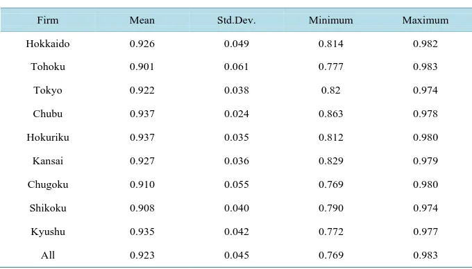
issatisfied only in some samples. For Model D, Table 4 reports some descriptive statistics for the estimates of
the cost efficiencies for each power utility. The cost efficiencies are calculated as exp
(
−uit)
, using the esti- mates of the inefficiency terms. The cost efficiencies range from 0 to 1, with larger values of cost efficiency meaning a firm is more efficient. The largest value of cost efficiency is 0.983 (Tohoku Electric), while the smallest value is 0.769 (Chugoku Electric). All values of the average cost efficiency for each electricity com- pany exceed 0.9. This suggests that all companies are quite cost efficient.In choosing among the usual panel models (Models A, B, and C), the fixed-effects model (Model) C is supported since the F test testing the null hypothesis that individual fixed effects are absent rejects the pooling models with a p-value of 0.000, and the log likelihood of the fixed-effects model is the largest among the usual panel models. LIMDEP 10 could not obtain the result of the Hausman test because the inverse of the covariance matrix for Hausman test could not be calculated. In the fixed-effect model, the assumption that the cost function is an increasing function in y1it,y2it,p1it,p2it, and p3it is satisfied in the almost samples except for y2it.
Because the estimated coefficient of nuclear power is negative and significant in Model C, the use of nuclear power seems to have contributed to reducing costs. Because the estimated coefficient of new energy is positive and significant in Model C, the use of new energy seems to increase costs.
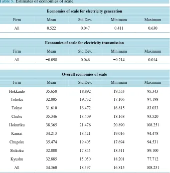
Estimates from the fixed effects model (Model C) are used to determine whether economies of scale exist and
whether economies of scope exist Table 5 reports some descriptive statistics for the estimates of economies of
[image:10.595.127.467.527.721.2]scale. Since the mean of the estimates of s1it for each power utility is under 1, these results suggest that econo-
Table 4.Estimates of r cost efficiencies: descriptive statistics.
Firm Mean Std.Dev. Minimum Maximum Hokkaido 0.926 0.049 0.814 0.982
Tohoku 0.901 0.061 0.777 0.983
Tokyo 0.922 0.038 0.82 0.974
Chubu 0.937 0.024 0.863 0.978
Hokuriku 0.937 0.035 0.812 0.980
Kansai 0.927 0.036 0.829 0.979
Chugoku 0.910 0.055 0.769 0.980
Shikoku 0.908 0.040 0.790 0.974
Kyushu 0.935 0.042 0.772 0.977
Table 5.Estimates of economies of scale.
Economies of scale for electricity generation
Firm Mean Std.Dev. Minimum Maximum
All 0.522 0.047 0.411 0.630
Economies of scale for electricity transmission
Firm Mean Std.Dev. Minimum Maximum
All −0.098 0.046 −0.214 0.014
Overall economies of scale
Firm Mean Std.Dev. Minimum Maximum Hokkaido 35.658 18.892 19.553 95.343
Tohoku 32.805 19.732 17.106 97.198 Tokyo 31.610 16.472 16.815 83.033 Chubu 35.346 18.409 18.168 93.520 Hokuriku 38.365 21.476 20.890 108.251
Kansai 34.213 18.421 19.016 94.478 Chugoku 35.474 19.405 17.694 94.531 Shikoku 32.888 17.845 18.511 89.100 Kyushu 32.885 15.050 18.201 77.712 All 34.360 18.397 16.815 108.251
mies of scope exist in the generation sector. The problem is that the mean estimates of s2it for each power
utility is negative. One possible reason for this is that the cost of transmission includes investment in plant and
equipment. Since the mean of the estimates of the ovrall economies of scale, SCLit, for each power utility is
over 1, these results suggest that overall economies of scope does not exist.
Figure 2 displays estimates of the overall economies of scale for each power utility from 1970 to 2010.
Movements of the overall economies of scale for all companies are more or less the same during the period. In
the 1970s, SCLit declined rapidly, and then, SCLit has been increasing slowly. The estmated value of SCLit
exceeds 1 throughout the period. Though this means that overall economies scale have not been existed during this period, the econoies of scales for generation and transmission was improved in the 1970s. In the 1970s, Japan started to convert to nuclear power in earnest after the oil shock. It is considered that the saving on oil use contributed to the economies of scales.
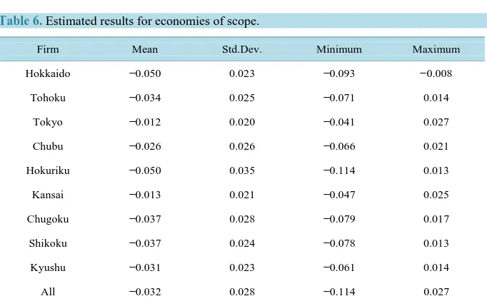
Table 6 reports some descriptive statistics for estimates of SCP12 for each power utility. Since the mean of
the estimates of SCP12 for each power utility is negative, these results suggest that economies of scope exist
between the generation sector and tranmission sector for electricity on average.
6. Concluding Remarks
Figure 2.Overall economies of scale over time.
Table 6. Estimated results for economies of scope.
Firm Mean Std.Dev. Minimum Maximum Hokkaido −0.050 0.023 −0.093 −0.008
Tohoku −0.034 0.025 −0.071 0.014 Tokyo −0.012 0.020 −0.041 0.027 Chubu −0.026 0.026 −0.066 0.021 Hokuriku −0.050 0.035 −0.114 0.013 Kansai −0.013 0.021 −0.047 0.025 Chugoku −0.037 0.028 −0.079 0.017 Shikoku −0.037 0.024 −0.078 0.013 Kyushu −0.031 0.023 −0.061 0.014
All −0.032 0.028 −0.114 0.027
in the electricity generation and distribution sectors. The structural separation of the transmission sector of elec-tricity from the generation of electric power, which has been discussed recently, is one example of a further lib-eralization. However, considering the existence of the scope of economies between the generation sector and the transmission sector, other kinds of liberalization should be introduced.
Acknowledgements
I would like to thank Hiroki Kawai, Colin McKenzie, Ryo Nakajima, Tatsuo Tanaka, and two anonymous refe-rees for their helpful comments and suggestions.
References
[1] Taniguchi, M. (2013) The Impact of Liberalization on the Production of Electricity in Japan, Keio/Kyoto Joined Global Center of Excellence Program, Raising Market Quality-Integrated Design of Market Infrastructure, DP2012-027.
http://ies.keio.ac.jp/old_project/old/gcoe-econbus/pdf/dp/DP2012-027.pdf
[2] Taniguchi, M. (2013) The Impact of Liberalization on the Production of Electricity in Japan. The Proceedings of the International Conference on Applied Economics (ICOAE) 2013, Istanbul, 27-29 June 2013, 712-721.
http://www.sciencedirect.com/science/article/pii/S221256711300083X
[3] Goto, M. and Inoue, T. (2012) Economic Analysis of Structural Reforms of Electricity Industry: Investigation of Cost Structure of Japanese Electricity (Denkijigyou no KouzoukaikakunikansuruKeizaiseibunseki: WagakuniDenkijigyou no Hiyoukouzoubunseki). Central Research Institute of Electric Power Industry Research Report, Paper#Y11009. (in Japanese)
http://criepi.denken.or.jp/jp/kenkikaku/report/download/PwquwpH8FPLMWnKfJ2Cyy0CZVgAfsMNW/report.pdf
[4] Kuwabara, T. and Ida, T. (2000) The Panel Data Analysis of the Japanese Electric Power Industry (Nihon no
0 20 40 60 80 100 120
1970 1972 1974 1976 1978 1980 1982 1984 1986 1988 1990 1992 1994 1996 1998 2000 2002 2004 2006 2008 2010
Hokkaido Tohoku Tokyo Chubu Hokuriku
Denryokusangyou no Panerudeta Bunseki), Kouekijigyoukenkyu. KouekiJigyouKenkyuu, 52, 71-82. (in Japanese)
[5] Nemoto, J. and Goto, M. (2006) Measurement of Technical and Allocative Efficiencies Using a CES Cost Frontier: A Benchmarking Study of Japanese Transmission-Distribution Electricity. Empirical Economics, 31, 31-48.
http://dx.doi.org/10.1007/s00181-005-0013-x
[6] Kinugasa, T. (2011) Estimating the Degree of Market Competitiveness after Deregulation: An Analysis Using the Translog Production Function for the Japanese Electricity Industry (Kiseikanwago no Shijoukyousoudo no Suitei; Ni-hon no Denryoku sangyou no Toransurogugata seisan kansuuwomotiita Bunseki). Proceedings of the 68thConference of Japan Economic Policy Association, Tokyo, 28-29 May 2011. (in Japanese)
http://www.komazawa-u.ac.jp/files/880/p37.pdf
[7] Tsutsui, M (2000) Comparison of Intertemporal Technical Efficiency by Sector among Japanese and US Electric Utili-ties. The Application of Malmquist Index Calculated by DEA, Central Research Institute of Electric Power Industry Research Report, Y99013. (in Japanese with English Abstract)
http://criepi.denken.or.jp/jp/kenkikaku/report/download/WUUZBO5d2c4xbfSn82i8CLzwTUZZUQYA/report.pdf
[8] Hattori, T., Jamasb, T. and Pollitt, M. (2005) Electricity Distribution in the UK and Japan: A Comparative Efficiency Analysis 1985-1998. Energy Journal, 26, 23-47. http://dx.doi.org/10.5547/ISSN0195-6574-EJ-Vol26-No2-2
[9] Yamaguchi, S. (2007) The Results and Issues of the Electricity Liberalizations in Japan: A Comparison of Japan to Europe and the US (Denryokujiyuuka no Seika to Kadai: Oubei to Nihon no Hikaku), Issue Brief, No. 595 (in Japanese)
http://www.ndl.go.jp/jp/data/publication/issue/0595.pdf
[10] Minister of Economy, Trade and Industry (2011) Material 3: Discussion Points of the Calculations for Electricity Charges (Shiryou 3: DenkiryoukinSanteijou no KakuRontennitsuite). Constructed by Heisei 23 nen 12 gatsu Denki-ryoukinseido Unyou no Minaoshinikakaru Yushikisyakaigi Jimukyoku.
http://www.meti.go.jp/committee/kenkyukai/energy/denkiryoukin/003_03_01.pdf
[11] Baumol, W.J., Panzar, J.C. and Willig, R.D. (1982) Contestable Markets and the Theory of Industry Structure. Har-court Brace Jovanovich, New York.
[12] Battese, G.E. and Coelli, T.J. (1992) Frontier Production Functions, Technical Efficiency and Panel Data: With Appli-cation to Paddy Farmers in India. Journal of Productivity Analysis, 3, 153-169.
http://dx.doi.org/10.1007/BF00158774
[13] Greene, W. (2005) Fixed and Random Effects in Stochastic Frontier Models. Journal of Productivity Analysis, 23, 7-35.