http://dx.doi.org/10.4236/pos.2014.51003
Satellite Clock Error and Orbital Solution Error
Estimation for Precise Navigation Applications
Bharati Bidikar1, Gottapu Sasibhushana Rao2, Laveti Ganesh3, MNVS Santosh Kumar4
1
Department of ECE,Andhra University, Visakhapatnam, India; 2Department of ECE,Andhra University, Visakhapatnam, India;
3
Department of ECE, ANITS, Visakhapatnam, India; 4Department of ECE, AITAM, Tekkali, India. Email: [email protected]
Received November 5th, 2013; revised December 5th, 2013; accepted December 12th, 2013
Copyright © 2014 Bharati Bidikar et al. This is an open access article distributed under the Creative Commons Attribution License, which permits unrestricted use, distribution, and reproduction in any medium, provided the original work is properly cited. In accor-dance of the Creative Commons Attribution License all Copyrights © 2014 are reserved for SCIRP and the owner of the intellectual property Bharati Bidikar et al. All Copyright © 2014 are guarded by law and by SCIRP as a guardian.
ABSTRACT
Global Positioning System (GPS) is a satellite-based navigation system that provides a three-dimensional user position (x,y,z), velocity and time anywhere on or above the earth surface. The satellite-based position accuracy is affected by several factors such as satellite clock error, propagation path delays and receiver noise due to which the GPS does not meet the requirements of critical navigation applications such as missile navigation and category I/II/III aircraft landings. This paper emphasizes on modelling the satellite clock error and orbital solu- tion (satellite position) error considering the signal emission time. The transmission time sent by each satellite in broadcast ephemerides is not accurate. This has to be corrected in order to obtain correct satellite position and in turn a precise receiver position. Signal transmission time or broadcast time from satellite antenna phase cen- ter is computed at the receiver using several parameters such as signal reception time, propagation time, pseu- dorange observed and satellite clock error correction parameters. This corrected time of transmission and broadcast orbital parameters are used for estimation of the orbital solution. The estimated orbital solution was validated with the precise ephemerides which are estimated by Jet Propulsion Laboratory (JPL), USA. The er- rors are estimated for a typical day data collected on 11th March 2011 from dual frequency GPS receiver located at Department of Electronics and Communication Engineering, Andhra University College of Engineering, Vi- sakhapatnam (17.73˚N/83.319˚E).
KEYWORDS
Satellite Clock Error; Satellite Clock Offset; Orbital Solution; Broadcast Ephemerides
1. Introduction
GPS has been widely used for precise positioning and na- vigation applications. In addition to the propagation er- rors, the receiver position accuracy, availability, reliabil-ity and integrreliabil-ity of GPS navigation solution are affected by satellite clock errors and orbital solution errors. Indi- vidual satellite clocks, although highly stable, may devi- ate from GPS system time. Hence for precise navigation applications, satellite clock error needs to be corrected.
In this paper, the satellite signal time of transmission is precisely estimated by considering the clock correction parameters like satellite clock bias (a0), satellite clock
drift (a1), satellite clock drift rate (a2), transmitted as part
of the navigation message, signal emission time at the antenna and the pseudorange measured between the sa- tellite and the receiver.
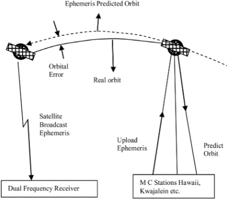
Figure 1. Satellite ephemeris errors.
are of high precision. The errors are estimated and ana- lysed for ephemeris data collected on 11th March 2011 at Department of Electronics and Communication Engineer- ing, Andhra University College of Engineering, Vishak- hapatnam.
2. Estimation of Satellite Clock Error and
Orbital Solution Error
The GPS receiver uses the same PRN codes which are transmitted by the 32 satellites for determining the dis-tance between each satellite and receiver. This disdis-tance is also known as pseudorange. For precise navigation solu-tion the computed pseudorange needs to be corrected for the errors like satellite clock error, tropospheric error, multipath errors, ionospheric errors etc. [1]. Among these the satellite clock error has a major impact on the pseu- dorange and is given by the following Equation (1)
sc m
P = +ρ ε ×C (1)
where, Pm= Measured range (meters); ρ= True range (meters); εsc
= Satellite clock error (sec); C= Velocity of light = 3 × 10⁸ meters/sec; from Equation (1) it is evi- dent that satellite clock error of 1 microsecond will lead to 300 meters error in the pseudorange [2].
2.1. Satellite Clock Error
All satellites contain atomic clocks that control all on-board timing operations, including broadcast signal gen-eration. Although, these clocks are highly stable still they lack of perfect synchronization between the timing of the satellite broadcast signals and GPS system time. Satellite
clock correction terms (a0, a1 and a2) and time of
clock toc, account for this lack of synchronization. All
these parameters are obtained from navigation file. The
on board clock stability is about 1 to 2 parts in 1013 over a period of one day [3]. These errors are common to all users observing the same satellite. The satellite clock er- ror is caused by the satellite oscillator not being synchro-nised to true time (GPS time).
The deviation of a particular clock from GPS system time is modeled as a quadratic function of time. The pa-rameters of this model are estimated, uploaded to the sa- tellite, and are broadcasted. The coefficients a0, a1
and a2 in the below equation are called the bias, drift,
and aging parameters of the satellite clock [4]. The esti-mation of satellite clock errors are as given below.
The satellite time of transmission is computed as
(
)
s rx
t =t − P c (2)
where, ts= satellite time of transmission (sec); trx= Signal reception time at receiver (sec); P = Pseudorange (meters); c = speed of light (meters/sec).
The time at which the signal received from the satellite and the pseudorange are read from the broadcast ephe-merides and observation data files respectively. The term
(
P c)
in Equation (2) gives the signal propagation time. This propagation time is subtracted from the signal re-ception time computed at the receiver and the residual time will be the instant at which the signal started from the satellite.The satellite clock offset
( )
dt is calculated as,s oc
dt= −t t (3)
where, ts= Satellite time of transmission (sec); toc = Time of clock (sec).
The satellite time of transmission is calculated using Equation (2) and time of clock is available in navigation
data.
The satellite clock error
( )
εsc is modelled using thesecond order polynomial as given below. The correction parameters bias, drift and aging are available in naviga- tion data.
2
0 1 2
sc
a a dt a dt
ε = + + (4)
where, a0= clock bias (sec); a1= clock drift (sec/sec);
2
a = frequency drift (i.e. aging) (sec/sec2); dt= satellite clock offset (sec).
The GPS time of transmission corresponds to the sig- nal emission time from the satellite and is computed as below,
sc GPS s
T = −t ε (5)
where, TGPS= Corrected GPS time of transmission (sec);
s
t = satellite time of transmission (sec); εsc= Satellite clock error (sec).
2.2. Broadcast Orbital Solution Error
The GPS navigation message file which contains the broadcast ephemerides gives the Keplerian parameters needed to compute the coordinates and clock correction for each satellite. This ephemeris data also contains the time information needed to correct that satellite’s clock to match with the GPS time. Error in satellite clock and orbital parameters results in estimation of incorrect orbit- al solution.
2.3. JPL Orbital Solution Interpolation
The Lagrange interpolation algorithm is used to find the intermediate values for the points (known as the data nodes) at a given interval. The precise satellite positions estimated by JPL for an epoch interval of 15 minutes where as broadcast satellite positions are estimated for an epoch interval of 15 seconds. The precise 3D satellite positions, Sk at different regular intervals of time are used
to interpolate the satellite positions in between the known intervals by using the Lagrange interpolation algorithm [5],
( )
1 1( )
2 2( )
n n( )
P x =y L x +y L x + + y L x (6)
where, L x L1
( ) ( )
, 2 x ,,Ln( )
x are Lagrange interpolat-ing polynomials defined as,
( )
(
)
(
)
1
1
1, 2,3, ,
n j j i n i j j
x x j i
L x i n
x x j i
= = − ≠ = = − ≠
∏
∏
(7)where, x = Lagrange multipliers; n = Number of inter-vals.
The above Lagrange interpolating polynomial for time interval t is written as the nth polynomial
( )
(
(
1)(
)(
2)(
)(
3) (
) (
1)
)
1 2 3 1
n n
n n n n n
t t t t t t t t L t
t t t t t t t t
− − − − − − = − − − −
These calculated polynomials are substituted in Equa-tion (6) to get the interpolated precise satellite posiEqua-tions.
3. Results and Discussion
The satellite clock errors and orbital solution errors are estimated and the analysis of the error which are support- ed by the relevant graphs and the tables are presented in this paper.
The broadcast orbital solution error and satellite clock error are estimated using the data collected by the recei- ver from 02:00 hours to 02:39 hours with an epoch inter- val of 15 seconds. During this observation period of 39 minutes (total of 157 epochs) out of 31 satellites, 9 (02, 05, 12, 15, 18, 21, 25, 26, 29) satellites were visible. Though the errors are computed and analyzed for all the
visible satellites, the results corresponding to a particular Satellite Vehicle Pseudo Random Noise (SVPRN 26) are presented in this paper. To compute the positional error of the satellite, the positions estimated by the receiver are compared with the one estimated by JPL, assuming the JPL estimates are of high precision.The precise epheme- rides estimated by JPL are interpolated using the Lag- range interpolation algorithm to generate satellite posi-tion for SVPRN 26 for 157 epochs with an epoch interval of 15 seconds. Tables given in this paper details 10 epo- chs of data and figures are plotted for 157 epochs.
The broadcast ephemerides are collected on 11th March 2011 from the dual frequency GPS receivers located at De- partment of Electronics and Communication, Andhra Uni- versity College of Engineering, Visakhapatnam (17.73˚N/ 83.319˚E). The precise ephemerides are collected from Jet Propulsion Laboratory (JPL), USA for the same day.
[image:3.595.307.538.559.732.2]3.1. Satellite Clock Error
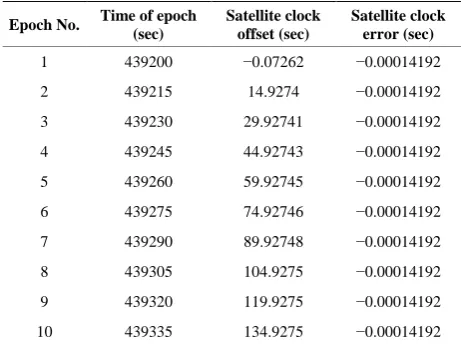
Table 1 details the satellite clock offset and satellite clock error of SVPRN26 for 10 epochs. Figure 2 and
Figure 3 shows these variations over 157 epoch and it is observed that the satellite clock offset is varied from −0.07262 to 2340 seconds and the corresponding clock
error is varied from −0.00014192 to −0.00014194 se-
conds.
3.2. Orbital Solution Error
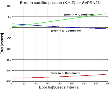
Table 2 details the error in each of the coordinates of the broadcast satellite position with that of the precise satel-lite position of SVPRN26 for 10 epochs. Figure 4 shows this variation over 157 epochs and it is observed that the satellite positions in the x-coordinate is deviated by 17.02 to −5.939 meters. Similarly, the error is varied from 2.973 to 63.89 meters and −235.8 to −218.1 meters for y- and z-coordinates respectively.
Table 1. Satellite clock offset and error of SVPRN 26.
Epoch No. Time of epoch (sec)
Satellite clock offset (sec)
Satellite clock error (sec)
1 439200 −0.07262 −0.00014192
2 439215 14.9274 −0.00014192
3 439230 29.92741 −0.00014192
4 439245 44.92743 −0.00014192
5 439260 59.92745 −0.00014192
6 439275 74.92746 −0.00014192
7 439290 89.92748 −0.00014192
8 439305 104.9275 −0.00014192
9 439320 119.9275 −0.00014192
Figure 2. Satellite clock offset for SVPRN 26.
[image:4.595.61.284.302.487.2]Figure 3. Satellite clock error for SVPRN26.
Table 2. Orbital solution error for SVPRN 26.
Epoch No. Time of epoch(s)
Orbital solution error (X,Y,Z) SVPRN 26 (m)
1 439200 17.018 2.973 −235.762
2 439215 16.799 3.351 −235.716
3 439230 16.581 3.729 −235.670
4 439245 16.363 4.107 −235.623
5 439260 16.147 4.486 −235.574
6 439275 15.931 4.864 −235.525
7 439290 15.716 5.243 −235.475
8 439305 15.503 5.623 −235.424
9 439320 15.290 6.002 −235.372
10 439335 15.078 6.382 −235.320
4. Conclusions
This paper reveals the importance of the satellite clock error and the orbital solution error.
Figure 4. Orbital solution error for SVPRN 26.
Satellite clock error. Over 157 epochs of data analysed, it is observed that the satellite clock offset varied from −0.07262 to 2340 seconds and the corresponding clock error varied from −0.00014192 to −0.00014194 seconds. Hence the clock error estimation needs to be modeled for precision applications, (e.g. CAT I/II aircraft landings, missile navigation).
Broadcast Orbital Solution Errors.
The error in satellite positions inturn affects the accuracy of navigation solution. Broadcast satelliteposition varied from precise positions and the deviation in x-coordinate is 17.02 to −5.939 meters over 157 epochs. Similarly the error varied from 2.973 to 63.89 meters and −235.8 to
−218.1 meters for y- and z-coordinates respectively. These positional errors have significant effect on the critical ap- plications, (e.g. studies of the crustal dynamics of the earth).
Acknowledgements
The work undertaken in this paper is supported by Min-istry of Science and Technology, Department of Science and Technology (DST), Government of India, New Delhi, under Woman Scientist Scheme(WOS-A), Vide Saction letter No. SR/WOS-A/ET-04/2013.
REFERENCES
[1] M. Pratap and E. Per, “Global Positioning System: Signals, Measurements and Performance,” 2nd Edition, Ganga-Ja- muna Press, New York, 2006.
[2] E. L. Akim and D. A. Tuchin, “GPS Errors Statistical Analysis for Ground Receiver Measurements,” Keldysh Institute of Applied Mathematics, Russia Academy of Sci- ences, 2002.
[3] G. S. Rao, “Global Navigation Satellite Systems,” Mc
0 20 40 60 80 100 120 140 160
-500 0 500 1000 1500 2000 2500
Satellite clock offset for SVPRN26
Epochs[30secs Interval]
Error [se
cs]
0 20 40 60 80 100 120 140 160
-1.4195 -1.4194 -1.4194 -1.4193 -1.4192 -1.4192 -1.4191 -1.4191
-1.419x 10
-4 Satellite clock error for SVPRN26
Epochs[30secs Interval]
Error [se
cs]
0 20 40 60 80 100 120 140 160
-250 -200 -150 -100 -50 0 50 100
Error in satellite position (X,Y,Z) for SVPRN26
Epochs[30secs Interval]
Error [meters]
Error in z- Coordinate Error in x- Coordinate
[image:4.595.56.287.533.682.2]Graw-Hill Education, New Delhi, 2010.
[4] E. D. Kaplan, “Understanding GPS: Principles and Appli- cations,” 2nd Edition, Artech House Publishers, Boston,
2006.